21 Wilcoxon-Mann-Whitney test

The Wilcoxon-Mann-Whitney (WMW) test (sometimes called Mann-Whitney U test or Wilcoxon Rank Sum test) is used to compare two independent samples and is often considered the non-parametric alternative to the Student’s t-test when there is violation of normality or for small sample sizes. However, if the samples are very small (both smaller than four observations) then statistical significance is impossible.

When we have finished this Chapter, we should be able to:

Learning objectives

Applying hypothesis testing
Compare two independent samples applying Wilcoxon-Mann-Whitney test
Interpret the results

21.1 Research question and Hypothesis Testing

We consider the data in thromboglobulin dataset that contains the urinary \(\beta\) thromboglobulin excretion (pg/ml) measured in 12 non-diabetic patients and 12 diabetic patients. The researchers used \(\alpha\) = 0.05 significance level to test if the distribution of urinary \(\beta\) thromboglobulin (b_TG) differs in the two groups.

Null hypothesis and alternative hypothesis

\(H_0\): the distribution of urinary \(\beta\) thromboglobulin is the same in the two groups
\(H_1\): the distribution of urinary \(\beta\) thromboglobulin is different in the two groups

NOTE: The null hypothesis is that the observations from one group do not tend to have higher or lower ranks than observations from the other group. This test does not compare the medians of the data as is commonly thought, it tests the whole distribution. However, if the distributions of the two groups have similar shapes and spreads (i.e., differing only in location), the WMW test can address (in most cases) whether there are differences in the medians between the two groups.(ref.)

21.2 Packages we need

We need to load the following packages:

# packages for graphs
library(ggrain)
library(ggsci)
library(ggpubr)

# packages for data description, transformation and analysis
library(dlookr)
library(rstatix)
library(sjstats)
library(here)
library(tidyverse)

# packages for reporting the results
library(gtsummary)
library(report)

21.3 Preparing the data

We import the data thromboglobulin in R:

library(readxl)
tg <- read_excel(here("data", "thromboglobulin.xlsx"))

Figure 21.1: Table with data from “depression” file.

We inspect the data and the type of variables:

glimpse(tg)

Rows: 24
Columns: 2
$ status <chr> "non_diabetic", "non_diabetic", "non_diabetic", "non_diabetic",…
$ b_TG   <dbl> 4.1, 6.3, 7.8, 8.5, 8.9, 10.4, 11.5, 12.0, 13.8, 17.6, 24.3, 37…

The data set tg has 24 patients (rows) and includes two variables (columns). The numeric (<dbl>) b_TG variable and the character (<chr>) status variable which should be converted to a factor (<fct>) variable using the factor() function as follows:

tg <- tg %>% 
  mutate(status = factor(status))
glimpse(tg)

Rows: 24
Columns: 2
$ status <fct> non_diabetic, non_diabetic, non_diabetic, non_diabetic, non_dia…
$ b_TG   <dbl> 4.1, 6.3, 7.8, 8.5, 8.9, 10.4, 11.5, 12.0, 13.8, 17.6, 24.3, 37…

21.4 Explore the characteristics of distribution for each group and check for normality

The distributions can be explored visually with appropriate plots. Additionally, summary statistics and significance tests to check for normality (e.g., Shapiro-Wilk test) can be used.

Graph

We can visualize the distribution of b_TG for the two groups:

ggplot(tg, aes(x= status, y = b_TG, fill = status)) +
  geom_rain(likert= TRUE, seed = 123, point.args = list(alpha = 0.3)) +
  theme_classic(base_size = 20) +
  labs(title = "Grouped Raincloud Plot:  Thromboglobulin by status") +
  scale_fill_jco() +
  theme(legend.position = "none",
        axis.text = element_text(size = 20))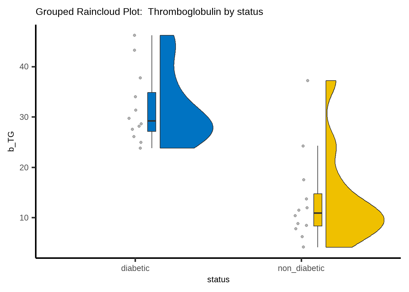

The above figure shows that the data in both groups are positively skewed and they have similar shaped distributions.

tg %>%
  ggqqplot("b_TG", color = "status", conf.int = F) +
  theme_classic(base_size = 20) +
  scale_color_jco() +
  facet_wrap(~ status) + 
  theme(legend.position = "none", 
        axis.text = element_text(size = 18))

Figure 21.3: Normality Q-Q plot for HDRS for paroxetine and placebo.

Summary statistics

The b_TG summary statistics for each group are:

Summary statistics by group

dplyr
dlookr

tg %>%
  group_by(status) %>%
  dplyr::summarise(
    n = n(),
    na = sum(is.na(b_TG)),
    min = min(b_TG, na.rm = TRUE),
    q1 = quantile(b_TG, 0.25, na.rm = TRUE),
    median = quantile(b_TG, 0.5, na.rm = TRUE),
    q3 = quantile(b_TG, 0.75, na.rm = TRUE),
    max = max(b_TG, na.rm = TRUE),
    mean = mean(b_TG, na.rm = TRUE),
    sd = sd(b_TG, na.rm = TRUE),
    skewness = EnvStats::skewness(b_TG, na.rm = TRUE),
    kurtosis= EnvStats::kurtosis(b_TG, na.rm = TRUE)
  ) %>%
  ungroup() |> 
  print(width = 100)

# A tibble: 2 × 12
  status           n    na   min    q1 median    q3   max  mean    sd skewness
  <fct>        <int> <int> <dbl> <dbl>  <dbl> <dbl> <dbl> <dbl> <dbl>    <dbl>
1 diabetic        12     0  23.8 27.2    29.2  34.8  46.2  31.8  7.17     1.05
2 non_diabetic    12     0   4.1  8.32   11.0  14.8  37.2  13.5  9.19     1.81
  kurtosis
     <dbl>
1    0.107
2    3.47

tg %>% 
  group_by(status) %>% 
  dlookr::describe(b_TG) %>% 
  select(described_variables,  status, n, na, mean, sd, p25, p50, p75, skewness, kurtosis) %>% 
  ungroup() |> 
  print(width = 100)

# A tibble: 2 × 11
  described_variables status           n    na  mean    sd   p25   p50   p75
  <chr>               <fct>        <int> <int> <dbl> <dbl> <dbl> <dbl> <dbl>
1 b_TG                diabetic        12     0  31.8  7.17 27.2   29.2  34.8
2 b_TG                non_diabetic    12     0  13.5  9.19  8.32  11.0  14.8
  skewness kurtosis
     <dbl>    <dbl>
1     1.05    0.107
2     1.81    3.47

The means are not very close to the medians (31.8 vs 29.2 and 13.5 vs 11.0). Moreover, both the skewness (1.81) and the (excess) kurtosis (3.47) for the non-diabetic group falls outside of the acceptable range of [-1, 1] indicating right-skewed and leptokurtic distribution.

Normality test

The Shapiro-Wilk test for normality for each group is:

tg %>%
  group_by(status) %>%
  shapiro_test(b_TG) %>% 
  ungroup()

# A tibble: 2 × 4
  status       variable statistic      p
  <fct>        <chr>        <dbl>  <dbl>
1 diabetic     b_TG         0.886 0.105 
2 non_diabetic b_TG         0.817 0.0148

We can see that the data for the non-diabetic group is not normally distributed (p=0.015 <0.05) according to the Shapiro-Wilk test.

21.5 Run the Wilcoxon-Mann-Whitney test

The difference in location between two distributions with similar shapes (Figure 21.2) can be tested using the Wilcoxon-Mann-Whitney (WMW) test:

Wilcoxon-Mann-Whitney test

Base R
rstatix

wilcox.test(b_TG ~ status, conf.int = T, data = tg)


    Wilcoxon rank sum exact test

data:  b_TG by status
W = 134, p-value = 0.0001028
alternative hypothesis: true location shift is not equal to 0
95 percent confidence interval:
 13.7 24.0
sample estimates:
difference in location 
                 18.95

Historical Note: As you can see, in R the Mann-Whitney test is calculated with the wilcox.test() function and it is called Wilcoxon rank-sum test. What is the reason for this? Henry Mann and Donald Whitney (1947) reported in their article that the test was first proposed by Frank Wilcoxon (1945) and they gave their version for the test. So the right would be to call this test Wilcoxon-Mann-Whitney (WMW) test.

tg |>
  wilcox_test(b_TG ~ status, detailed = T) |> 
  print(width = 100)

# A tibble: 1 × 12
  estimate .y.   group1   group2          n1    n2 statistic        p conf.low
*    <dbl> <chr> <chr>    <chr>        <int> <int>     <dbl>    <dbl>    <dbl>
1     19.0 b_TG  diabetic non_diabetic    12    12       134 0.000103     13.7
  conf.high method   alternative
*     <dbl> <chr>    <chr>      
1        24 Wilcoxon two.sided

The result (the median of the difference¹ = 18.95, 95%CI: 13.7 to 24) is significant (p <0.001) and we reject the null hypothesis.

¹ Note: the estimator for the difference in location parameters does not estimate the difference in medians (a common misconception) but rather the median of the difference between the two samples.

In general, however, WMW test is regarded as a test of comparing the difference in ranks between the two groups as follows:

mwu(tg, b_TG, status, out = "browser")

Mann-Whitney U-Test
Groups	N	Mean Rank	Mann-Whitney U	Wilcoxon W	Z	Effect Size	p-value
diabetic non_diabetic	12 12	17.67 7.33	212	134	3.580	0.731	0.000

21.6 Present the results

Summary table

It is common practice to report the median (IQR) for each group in summary tables.

Show the code

tg %>% 
  tbl_summary(
    by = status, 
    statistic = b_TG ~ "{median} ({p25}, {p75})", 
    digits = list(everything() ~ 1),
    label = list(b_TG ~ "b_TG \n(pg/ml)"), 
    missing = c("no")) %>% 
  add_p(test = b_TG ~ "wilcox.test") %>% 
  add_n()

Characteristic	N	diabetic, N = 12¹	non_diabetic, N = 12¹	p-value²
b_TG (pg/ml)	24	29.3 (27.2, 34.9)	11.0 (8.3, 14.8)	<0.001
¹ Median (IQR)
² Wilcoxon rank sum exact test

Report the results

There is also a specific package with the name {report} that may be useful in reporting the results of WMW test:

report_results <- wilcox.test(tg$b_TG ~ tg$status) 
report(report_results)

Effect sizes were labelled following Funder's (2019) recommendations.

The Wilcoxon rank sum exact test testing the difference in ranks between
tg$b_TG and tg$status suggests that the effect is positive, statistically
significant, and very large (W = 134.00, p < .001; r (rank biserial) = 0.86,
95% CI [0.68, 0.94])

We can use the information to write up a final report:

Final report

There is evidence that the urinary \(\beta\) thromboglobulin excretion is higher in diabetic group, median = 29.2 (IQR: 27.1, 34.8) pg/ml, as compared to non-diabetic group, 10.9 (8.3, 14.8) pg/ml. The WMW test suggests that there is a significant difference in mean ranks between the two groups (17.67 Vs 7.33, p <0.001).