36 Measures of diagnostic test accuracy
When we have finished this Chapter, we should be able to:
36.1 Research questions
To estimate the diagnostic accuracy of digital mammography (index test) in the detection of breast cancer, using histopathology as a “gold standard” in women aged over 40 years, who are undergoing mammography for the evaluation of different symptoms related to breast diseases.
To estimate the post-test probability of breast cancer when the digital mammography is positive or negative given a pre-test probability.
36.2 Packages we need
We need to load the following packages:
36.3 Contingency 2x2 table
Generally, an individual’s disease status is a dichotomous variable; the individual either has the disease (
If the index test gives a dichotomous result for each participant in a study, the data can be tabulated in a 2 x 2 table of test result (
| Outcome according to the reference standard | ||||
|---|---|---|---|---|
|
(Disease present) |
(Disease absent) |
Totals | ||
| Index Test result | TP=890 | FP=110 | TP+FP=1000 | |
| FN=20 | TN=200 | TN+FN=220 | ||
| Totals | TP+FN=910 | TN+FP=310 |
N=1220 (TP+TN+FP+FN) |
where
TP: true positive; test positive and disease present (Test+ ∩ Outcome+)
FP = false positive; test positive and disease absent (Test+ ∩ Outcome-)
FN = false negative; test negative and disease present (Test- ∩ Outcome+)
TN = true negative; test negative and disease absent (Test- ∩ Outcome-)
36.4 Diagnostic Accuracy Measures
Basic Diagnostic Accuracy Measures
The Sensitivity (Se) of a diagnostic test refers to the ability of the test to correctly identify those individuals with the disease. It is defined as the proportion of true positive test results among individuals who have the disease.
Se =
The Specificity (Sp) of a diagnostic test refers to the ability of the test to correctly identify those patients without the disease. It is defined as the proportion of true negative test results among individuals who do not have the disease.
Sp =
Positive Predictive Value (PPV) is the probability that individuals with a positive diagnostic test result actually have the disease. It is defined as the proportion of true positive test results among individuals who have a positive test.
PPV =
Negative Predictive Value (NPV) is the probability that individuals with a negative diagnostic test result are truly free from the disease. It is defined as the proportion of true negative test results among individuals who have a negative test.
NPV =
Positive and negative predictive values are influenced by the prevalence of disease in the population that is being tested. Using the same test in a population with a higher prevalence (e.g. women over the age of 55) increases positive predictive value. Conversely, increased prevalence results in decreased negative predictive value. Therefore, when considering predictive values of diagnostic or screening tests, we should take into account the influence of the prevalence of the disease.
And other useful diagnostic measures are following:
More Diagnostic Accuracy Measures
Apparent prevalence is the proportion of individuals with a positive test result.
Apparent prevalence =
True prevalence is the proportion of individuals that are truly diseased.
True prevalence =
The Likelihood ratio for a positive test result (LR+) is the likelihood (probability) of an individual who has the disease testing positive divided by the likelihood (probability) of an individual who does not have the disease testing positive. It is calculated as sensitivity divided by 1 minus the specificity value.
LR+ =
The Likelihood ratio for a negative test result (LR-) is the probability of an individual who has the disease testing negative divided by the probability of an individual who does not have the disease testing negative. It is calculated as 1 minus the sensitivity divided by specificity value.
LR- =
Diagnostic accuracy (effectiveness), expressed as a proportion of correctly classified subjects (TP+TN) among all subjects (N). Diagnostic accuracy is affected by the disease prevalence.
Accuracy =
In R:
tb1 <- as.table(
  rbind(c(890, 110), c(20, 200))
  )

dimnames(tb1) <- list(
  Test = c("Test +", "Test -"),
  Outcome = c("Outcome +", "Outcome -")
)

tb1
Outcome
Test Outcome + Outcome -
Test + 890 110
Test - 20 200From this contingency table, we can create a basic mosaic plot.
mosaicplot(t(tb1), col = c("goldenrod1", "firebrick"),
           cex.axis = 0.9, main=NULL)
df <- reshape2::melt(tb1)

p <- ggplot(df) +
  geom_mosaic(aes(weight = value, x = product(Test, Outcome)),
              fill = c("goldenrod1", "firebrick",  "goldenrod1", "firebrick"))

df2 <- ggplot_build(p)$data[[1]][3:6]
Warning: The `scale_name` argument of `continuous_scale()` is deprecated as of ggplot2
3.5.0.Warning: The `trans` argument of `continuous_scale()` is deprecated as of ggplot2 3.5.0.
ℹ Please use the `transform` argument instead.Warning: `unite_()` was deprecated in tidyr 1.2.0.
ℹ Please use `unite()` instead.
ℹ The deprecated feature was likely used in the ggmosaic package.
Please report the issue at <https://github.com/haleyjeppson/ggmosaic>.df2$percentage <- round(100*df$value/sum(df$value), 2)
df2$lab <- paste0(df$value, " (", df2$percentage, "%", ")")
p + geom_label(data = df2,
aes(x = (xmin+xmax)/2, y = (ymin+ymax)/2, label = lab))
epi.tests(tb1, digits = 3) Outcome + Outcome - Total
Test + 890 110 1000
Test - 20 200 220
Total 910 310 1220
Point estimates and 95% CIs:
--------------------------------------------------------------
Apparent prevalence * 0.820 (0.797, 0.841)
True prevalence * 0.746 (0.720, 0.770)
Sensitivity * 0.978 (0.966, 0.987)
Specificity * 0.645 (0.589, 0.698)
Positive predictive value * 0.890 (0.869, 0.909)
Negative predictive value * 0.909 (0.863, 0.944)
Positive likelihood ratio 2.756 (2.371, 3.204)
Negative likelihood ratio 0.034 (0.022, 0.053)
False T+ proportion for true D- * 0.355 (0.302, 0.411)
False T- proportion for true D+ * 0.022 (0.013, 0.034)
False T+ proportion for T+ * 0.110 (0.091, 0.131)
False T- proportion for T- * 0.091 (0.056, 0.137)
Correctly classified proportion * 0.893 (0.875, 0.910)
--------------------------------------------------------------
* Exact CIs
Alternatively, we can obtain the same results in R using the diag_test2() function from the {pubh} package:
diag_test2(890, 110, 20, 200)36.5 Likelihood ratios in practice
36.5.1 Interpretation of LRs
Likelihood ratio (LR), along with sensitivity and specificity, can be considered properties of the test itself that do not change with the prevalence of disease.
In our example, LR+ = 2.756, meaning a positive result in digital mammography is approximately 2.8 times more likely to be a true positive test than a false positive test.
Similarly, LR- = 0.034, meaning a negative result in digital mammography is approximately 0.034 times more likely to be a false negative test than a true negative test. This can also be interpreted as: A woman without breast cancer is about 29.4 (= 1/0.034) times more likely to have a negative digital mammography test than a woman with breast cancer.
In clinical practice, a higher LR+ is desirable for tests used to “rule in” a disease, while a lower LR- is preferred for tests used to “rule out” the chance that the individual has the disease.
36.5.2 Application of LRs (revising the probability of disease)
The LR is commonly used in decision-making based on Bayes’ Theorem (Chapter 13). The pre-test odds of a particular diagnosis, multiplied by the likelihood ratio of the diagnostic test, determines the post-test odds.
These post-test odds provides an updated estimate of the odds that the patient has the condition or disease after taking into account the diagnostic test result. If the test result is positive, we use the LR+ for this calculation. If the test result is negative, we use the LR- instead. In both scenarios, the odds refer to the odds in favor of the disease being present.
Example: LR+
LR+ tells us how much the odds of the condition or disease being present increase given a positive test result.
LR+ greater than 1: Increases the post-test odds.
LR+ of 1: No change in the post-test odds (post-test odds equals pre-test odds).
Now, let’s suppose that, based on family history of breast cancer and clinical symptoms, a woman has 0.78 probability for breast cancer (pre-test probability).
We are interested in the the post-test probability of breast cancer when the digital mammography is positive. It is important to note that “odds” and “probability” are not the same; however, they can be derived from each other as follows:
The Fagan nomogram allows us to turn pre-test probabilities into post-test probabilities without needing to convert into odds. The nomogram typically consists of three parallel scales representing the pre-test probability, the likelihood ratio, and the post-test probability. We can visually estimate the post-test probability of a positive diagnosis result by drawing a line from the known pre-test probability, through the LR+ and read off the post-test probability.
In R:
fagan.plot(probs.pre.test = 0.78, LR = 2.756)
Example: LR-
LR- tells us how much the odds of the condition or disease being present decrease given a negative test result.
LR- less than 1: Decreases the post-test odds.
LR- of 1: No change in the probability (post-test odds equals pre-test odds).
What is the the post-test probability of breast cancer for the same population when the digital mammography is negative?
In R:
fagan.plot(probs.pre.test = 0.78, LR = 0.034)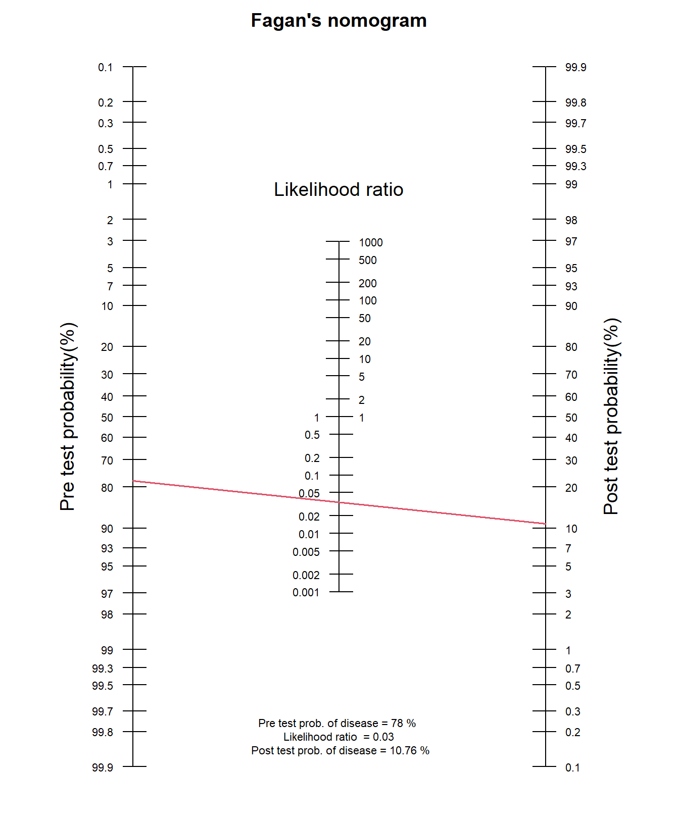
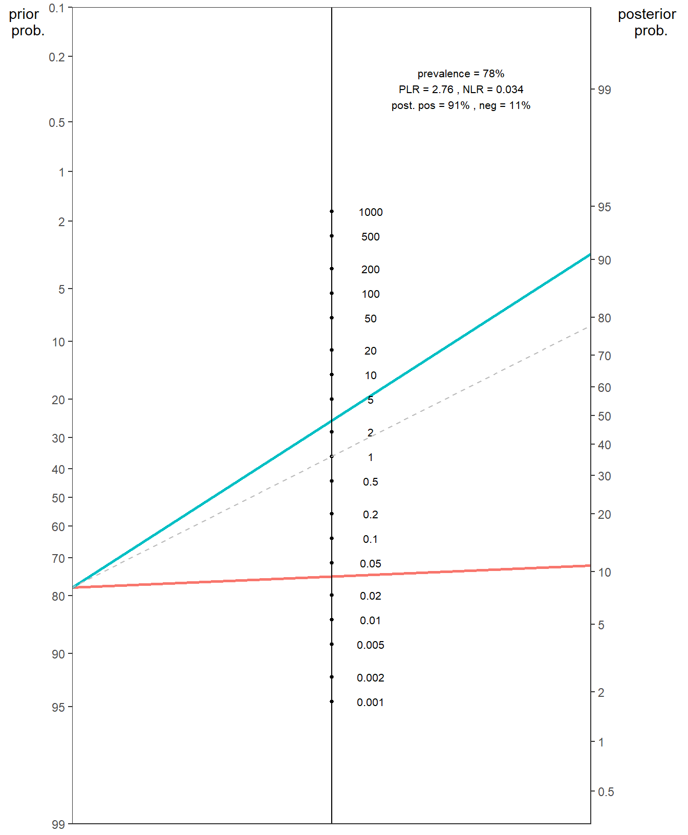
We can also use the epi.nomogram() and nomogrammer() functions which allow us to calculate the post-test probability and plot Fagan’s nomgrams with ggplot2, respectively:
epi.nomogram(se = NA, sp = NA, lr = c(2.755, 0.034), pre.pos = 0.78,
             verbose = FALSE)
Given a positive test result, the post-test probability of being outcome positive is 0.91
Given a negative test result, the post-test probability of being outcome positive is 0.11 # nomogrammer is a standalone function from the below repository
source("https://raw.githubusercontent.com/achekroud/nomogrammer/master/nomogrammer.r")
nomogrammer(Prevalence = 0.78,
Plr = 2.755,
Nlr = 0.034,
Detail = TRUE,
NullLine = TRUE)