26 One-way Repeated Measures ANOVA
The one-way repeated measures analysis of variance (also known as a within-subjects ANOVA) is an extension of the paired t-test designed to assess whether there are significant differences in the means of three or more related groups, such as comparing the difference between three or more time points.
26.1 Research question and Hypothesis Testing
Participants used margarine for 12 weeks. Their blood total cholesterol (TCH; in mmol/L) was measured before the special diet, after 6 weeks and after 12 weeks.
26.2 Packages we need
We need to load the following packages:
26.3 Preparing the data
We import the data cholesterol in R:
library(readxl)
dat_TCH <- read_excel(here("data", "cholesterol.xlsx"))We inspect the data and the type of variables:
glimpse(dat_TCH)Rows: 18
Columns: 3
$ week0 <dbl> 6.42, 6.76, 6.56, 4.80, 8.43, 7.49, 8.05, 5.05, 5.77, 3.91, 6.7…
$ week6 <dbl> 5.83, 6.20, 5.83, 4.27, 7.71, 7.12, 7.25, 4.63, 5.31, 3.70, 6.1…
$ week12 <dbl> 5.75, 6.13, 5.71, 4.15, 7.67, 7.05, 7.10, 4.67, 5.33, 3.66, 5.9…26.4 Assumptions
A. Explore the characteristics of distribution for each time point and check for normality
The distributions can be explored visually with appropriate plots. Additionally, summary statistics and significance tests to check for normality (e.g., Shapiro-Wilk test) can be used.
Graphs
We can visualize the distribution of cholesterol for the three time points:
dat_TCH_long <- dat_TCH |>
  mutate(id = row_number()) |>
  pivot_longer(cols = -id, names_to = "time", values_to = "cholesterol") |>
mutate(time = factor(time, levels = c("week0", "week6", "week12")))ggplot(dat_TCH_long, aes(x= time, y = cholesterol, fill = time)) +
geom_rain(likert= TRUE, seed = 123, point.args = list(alpha = 0.3)) +
#theme_prism(base_size = 14, base_line_size = 0.4, palette = "office") +
labs(title = "Grouped Raincloud Plot: Cholesterol by time point") +
scale_fill_jco() +
theme(legend.position = "none")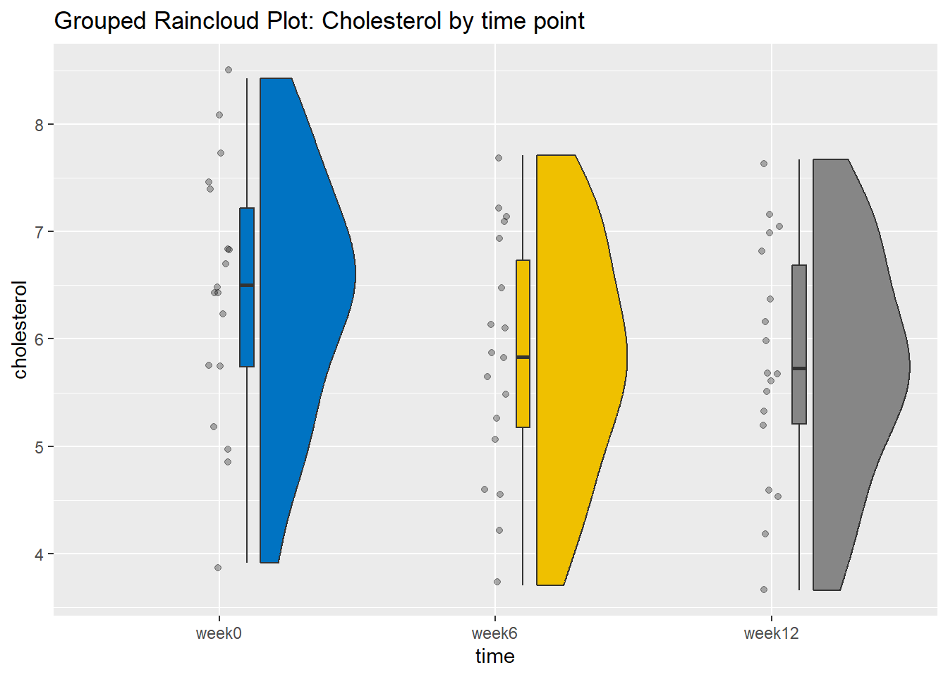
ggqqplot(dat_TCH_long, "cholesterol", color = "time", conf.int = F) +
  #theme_prism(base_size = 14, base_line_size = 0.4, palette = "office") +
  scale_color_jco() +
  facet_wrap(~ time) +
  theme(legend.position = "none")
The above figures show that the data are close to symmetry and the assumption of a normal distribution is reasonable.
Summary statistics
The cholesterol summary statistics for each time point are:
cholesterol_summary <- dat_TCH_long %>%
  group_by(time) %>%
  dplyr::summarise(
    n = n(),
    na = sum(is.na(cholesterol)),
    min = min(cholesterol, na.rm = TRUE),
    q1 = quantile(cholesterol, 0.25, na.rm = TRUE),
    median = quantile(cholesterol, 0.5, na.rm = TRUE),
    q3 = quantile(cholesterol, 0.75, na.rm = TRUE),
    max = max(cholesterol, na.rm = TRUE),
    mean = mean(cholesterol, na.rm = TRUE),
    sd = sd(cholesterol, na.rm = TRUE),
    skewness = EnvStats::skewness(cholesterol, na.rm = TRUE),
    kurtosis= EnvStats::kurtosis(cholesterol, na.rm = TRUE)
  ) %>%
  ungroup()

cholesterol_summary
# A tibble: 3 × 12
time n na min q1 median q3 max mean sd skewness kurtosis
<fct> <int> <int> <dbl> <dbl> <dbl> <dbl> <dbl> <dbl> <dbl> <dbl> <dbl>
1 week0 18 0 3.91 5.74 6.5 7.22 8.43 6.41 1.19 -0.311 -0.248
2 week6 18 0 3.7 5.18 5.83 6.73 7.71 5.84 1.12 -0.171 -0.708
3 week… 18 0 3.66 5.21 5.73 6.69 7.67 5.78 1.10 -0.188 -0.561dat_TCH_long |>
group_by(time) |>
dlookr::describe(cholesterol) |>
select(described_variables, time, n, mean, sd, p25, p50, p75, skewness, kurtosis) |>
ungroup() |>
print(width = 100)Registered S3 methods overwritten by 'dlookr':
method from
plot.transform scales
print.transform scales# A tibble: 3 × 10
described_variables time n mean sd p25 p50 p75 skewness
<chr> <fct> <int> <dbl> <dbl> <dbl> <dbl> <dbl> <dbl>
1 cholesterol week0 18 6.41 1.19 5.74 6.5 7.22 -0.311
2 cholesterol week6 18 5.84 1.12 5.18 5.83 6.73 -0.171
3 cholesterol week12 18 5.78 1.10 5.21 5.73 6.69 -0.188
kurtosis
<dbl>
1 -0.248
2 -0.708
3 -0.561The means are close to medians and the standard deviations are also similar. Moreover, both skewness and (excess) kurtosis falls into the acceptable range of [-1, 1] indicating approximately normal distributions for all time points.
Normality test
dat_TCH_long |>
  group_by(time) |>
  shapiro_test(cholesterol) |>
  ungroup()
# A tibble: 3 × 4
time variable statistic p
<fct> <chr> <dbl> <dbl>
1 week0 cholesterol 0.982 0.967
2 week6 cholesterol 0.977 0.912
3 week12 cholesterol 0.977 0.918The tests of normality suggest that the data for the cholesterol in all time points are normally distributed (p > 0.05).
In our example, the data at each time point are approximately normally distributed; a repeated ANOVA analysis can be performed.
B. Sphericity test for equality of variances of the differences
In addition, the assumption of sphericity must be met for accurate interpretation of the results of repeated ANOVA. This assumption is usually checked with the Mauchly’s sphericity test, wherein null hypothesis states that the variances of the differences are equal.
MauchlySphericityTest(dat_TCH)[1] 0.0004439621Here the assumption of sphericity has not been met (p < 0.001). In this case, we have to correct the degrees of freedom in repeated ANOVA analysis.
26.5 Run the one-way repeated ANOVA test
First, let’s run the repeated ANOVA test without any correction:
repeated_anova <- dat_TCH_long |>
  anova_test(dv = cholesterol, wid = id, within = time)

repeated_anova[1]
$ANOVA
Effect DFn DFd F p p<.05 ges
1 time 2 34 212.321 6.17e-20 * 0.061However, we must adjust the results of the repeated ANOVA analysis. The correction involves multiplying the degrees of freedom DFn=2 and DFd=34 by a quantity e, which measures the extent to which the data deviates from ideal sphericity (e ranges between 0 and 1, where 1 indicates no departure from sphericity). Two methods are commonly used for calculating e:
- the correction of Greenhouse-Geisser (GGe).
- the correction of Huynh-Feldt (HFe).
In R, we can calculate both GGe and HFe, as follows:
repeated_anova[3]$`Sphericity Corrections`
Effect GGe DF[GG] p[GG] p[GG]<.05 HFe DF[HF] p[HF] p[HF]<.05
1 time 0.618 1.24, 21 3.89e-13 * 0.642 1.28, 21.82 1.44e-13 *The general recommendation is to use the Greenhouse-Geisser correction when GGe is less than 0.75; otherwise, we should use the Huynh-Feldt correction HFe.
As the GGe value is less than 0.75, we use the Greenhouse-Geisser adjustment of 0.618. The corrected degrees of freedom are:
and
The new p-value (p[GG]) is available next to the corrected degrees of freedom (DF[GG]). In this example, as p<0.001 there is evidence of a difference between at least two time points.
By utilizing the get_anova_table() function to extract the ANOVA table, the Greenhouse-Geisser sphericity correction is automatically applied when the assumption of sphericity is violated.
get_anova_table(repeated_anova)ANOVA Table (type III tests)
Effect DFn DFd F p p<.05 ges
1 time 1.24 21 212.321 3.89e-13 * 0.061