24 One-way ANOVA test

One-way analysis of variance, usually referred to as one-way ANOVA, is a statistical test used when we want to compare several means. We may think of it as an extension of Student’s t-test to the case of more than two independent samples.

Although, this test can detect a difference between several groups it does not inform us about which groups are different from the others. At first glance, we might think to compare all groups in pairs with multiple t-tests. However, this procedure may lead to incorrect conclusions (known as multiple comparisons problem) because each comparison increases the likelihood of committing at least one Type I error within a set of comparisons (familly-wise Type I error rate).

This is the reason why, after an ANOVA test concluding on a significant difference between group means, we should not just compare all possible pairs of groups with t-tests. Instead we perform statistical tests that take into account the number of planned comparisons (post hoc tests) and make the necessary adjustments to ensure that Type I error is not inflated.

When we have finished this Chapter, we should be able to:

Learning objectives

Applying hypothesis testing
Compare more than two independent samples applying ANOVA
Perform post-hoc tests
Interpret the results

24.1 Research question and Hypothesis Testing

We consider the data in dataDWL dataset. In this example we explore the variations between weight loss according to four different types of diet. The question that may be asked is: does the average weight loss differ according to the diet?

Null hypothesis and alternative hypothesis

\(H_0\): all group means are equal (the means of weight loss in the four diets are equal; \(\mu_{1} = \mu_{2} = \mu_{3} = \mu_{4}\))
\(H_1\): at least one group mean differs from the others (there is at least one diet with mean weight loss different from the others)

24.2 Packages we need

We need to load the following packages:

library(rstatix)
library(PupillometryR)
library(gtsummary)
library(dabestr)

library(here)
library(tidyverse)

24.3 Preparing the data

We import the data dataDWL in R:

library(readxl)
dataDWL <- read_excel(here("data", "dataDWL.xlsx"))

Figure 24.1: Table with data from “dataDWL” file.

We inspect the data and the type of variables:

glimpse(dataDWL)

Rows: 60
Columns: 2
$ WeightLoss <dbl> 9.9, 9.6, 8.0, 4.9, 10.2, 9.0, 9.8, 10.8, 6.2, 8.3, 12.9, 1…
$ Diet       <chr> "A", "A", "A", "A", "A", "A", "A", "A", "A", "A", "A", "A",…

The dataset dataDWL has 60 participants and includes two variables. The numeric (<dbl>) WeightLoss variable and the character (<chr>) Diet variable (with levels “A”, “B”, “C” and “D”) which should be converted to a factor variable using the factor() function as follows:

dataDWL <- dataDWL %>% 
  mutate(Diet = factor(Diet))
glimpse(dataDWL)

Rows: 60
Columns: 2
$ WeightLoss <dbl> 9.9, 9.6, 8.0, 4.9, 10.2, 9.0, 9.8, 10.8, 6.2, 8.3, 12.9, 1…
$ Diet       <fct> A, A, A, A, A, A, A, A, A, A, A, A, A, A, A, B, B, B, B, B,…

24.4 Assumptions

Check if the following assumptions are satisfied

The data are normally distributed in all groups
The data in all groups have similar variance (also named as homogeneity of variance or homoscedasticity)

A. Explore the characteristics of distribution for each group and check for normality

The distributions can be explored visually with appropriate plots. Additionally, summary statistics and significance tests to check for normality (e.g., Shapiro-Wilk test) can be used.

Graphs

We can visualize the distribution of WeightLoss for the four Diet groups:

set.seed(123)
ggplot(dataDWL, aes(x=Diet, y=WeightLoss)) + 
  geom_flat_violin(aes(fill = Diet), scale = "count") +
  geom_boxplot(width = 0.14, outlier.shape = NA, alpha = 0.5) +
  geom_point(position = position_jitter(width = 0.05), 
             size = 1.2, alpha = 0.6) +
  ggsci::scale_fill_jco() +
  theme_classic(base_size = 14) +
  theme(legend.position="none", 
        axis.text = element_text(size = 14))

The above figure shows that the data are close to symmetry and the assumption of a normal distribution is reasonable. Additionally, we can observe that the largest weight loss seems to have been achieved by the participants in C diet.

Summary statistics

The WeightLoss summary statistics for each diet group are:

Summary statistics by group

dplyr
dlookr

DWL_summary <- dataDWL %>%
  group_by(Diet) %>%
  dplyr::summarise(
    n = n(),
    na = sum(is.na(WeightLoss)),
    min = min(WeightLoss, na.rm = TRUE),
    q1 = quantile(WeightLoss, 0.25, na.rm = TRUE),
    median = quantile(WeightLoss, 0.5, na.rm = TRUE),
    q3 = quantile(WeightLoss, 0.75, na.rm = TRUE),
    max = max(WeightLoss, na.rm = TRUE),
    mean = mean(WeightLoss, na.rm = TRUE),
    sd = sd(WeightLoss, na.rm = TRUE),
    skewness = EnvStats::skewness(WeightLoss, na.rm = TRUE),
    kurtosis= EnvStats::kurtosis(WeightLoss, na.rm = TRUE)
  ) %>%
  ungroup()

DWL_summary

# A tibble: 4 × 12
  Diet      n    na   min    q1 median    q3   max  mean    sd skewness kurtosis
  <fct> <int> <int> <dbl> <dbl>  <dbl> <dbl> <dbl> <dbl> <dbl>    <dbl>    <dbl>
1 A        15     0   4.9  8.15    9.6  10.5  12.9  9.18  2.30  -0.471    -0.302
2 B        15     0   3.8  7.85    9.2  10.8  12.7  8.91  2.78  -0.467    -0.515
3 C        15     0   8.7 10.8    12.2  13    15.1 12.1   1.79  -0.0451   -0.530
4 D        15     0   5.8  9.5    10.5  11.8  13.7 10.5   2.23  -0.475     0.229

dataDWL %>% 
  group_by(Diet) %>% 
  dlookr::describe(WeightLoss) %>% 
  select(described_variables,  Diet, n, mean, sd, p25, p50, p75, skewness, kurtosis) %>% 
  ungroup()

Registered S3 methods overwritten by 'dlookr':
  method          from  
  plot.transform  scales
  print.transform scales

# A tibble: 4 × 10
  described_variables Diet      n  mean    sd   p25   p50   p75 skewness
  <chr>               <fct> <int> <dbl> <dbl> <dbl> <dbl> <dbl>    <dbl>
1 WeightLoss          A        15  9.18  2.30  8.15   9.6  10.5  -0.471 
2 WeightLoss          B        15  8.91  2.78  7.85   9.2  10.8  -0.467 
3 WeightLoss          C        15 12.1   1.79 10.8   12.2  13    -0.0451
4 WeightLoss          D        15 10.5   2.23  9.5   10.5  11.8  -0.475 
# ℹ 1 more variable: kurtosis <dbl>

The means are close to medians and the standard deviations are also similar. Moreover, both skewness and (excess) kurtosis falls into the acceptable range of [-1, 1] indicating approximately normal distributions for all diet groups.

Normality test

The Shapiro-Wilk test for normality for each diet group is:

dataDWL %>%
  group_by(Diet) %>%
  shapiro_test(WeightLoss) %>% 
  ungroup()

# A tibble: 4 × 4
  Diet  variable   statistic     p
  <fct> <chr>          <dbl> <dbl>
1 A     WeightLoss     0.958 0.662
2 B     WeightLoss     0.941 0.390
3 C     WeightLoss     0.964 0.768
4 D     WeightLoss     0.944 0.435

The tests of normality suggest that the data for the WeightLoss in all groups are normally distributed (p > 0.05).

B. Levene’s test for equality of variances

The Levene’s test for equality of variances is:

dataDWL %>% 
  levene_test(WeightLoss ~ Diet)

# A tibble: 1 × 4
    df1   df2 statistic     p
  <int> <int>     <dbl> <dbl>
1     3    56     0.600 0.617

Since the p = 0.617 > 0.05, the null hypothesis (\(H_{0}\): the variances of WeighLoss in four diet groups are equal) can not be rejected.

24.5 Run the one-way ANOVA test

Now, we will perform an one-way ANOVA (with equal variances: Fisher’s classic ANOVA) to test the null hypothesis that the mean weight loss is the same for all the diet groups.

One-way ANOVA test

Base R
rstatix

# Compute the analysis of variance
anova_one_way <- aov(WeightLoss ~ Diet, data = dataDWL)

# Summary of the analysis
summary(anova_one_way)

            Df Sum Sq Mean Sq F value  Pr(>F)   
Diet         3  97.33   32.44   6.118 0.00113 **
Residuals   56 296.99    5.30                   
---
Signif. codes:  0 '***' 0.001 '**' 0.01 '*' 0.05 '.' 0.1 ' ' 1

dataDWL %>% 
  anova_test(WeightLoss ~ Diet, detailed = T)

ANOVA Table (type II tests)

  Effect   SSn     SSd DFn DFd     F     p p<.05   ges
1   Diet 97.33 296.987   3  56 6.118 0.001     * 0.247

The statistic F=6.118 indicates the obtained F-statistic = (variation between sample means \(/\) variation within the samples). Note that we are comparing to an F-distribution (F-test). The degrees of freedom in the numerator (DFn) and the denominator (DFd) are 3 and 56, respectively (numarator: variation between sample means; denominator: variation within the samples).

The p=0.001 is lower than 0.05. There is at least one diet with mean weight loss which is different from the others means.

From ANOVA table provided by the {rstatix} we can also calculate the generalized effect size (ges). The ges is the proportion of variability explained by the factor Diet (SSn) to total variability of the dependent variable (SSn + SSd), so:

\[\ ges= 97.33 / (97.33 + 296.987) = 97.33 / 394.317 = 0.247\] A ges of 0.247 (24.7%) means that 24.7% of the change in the weight loss can be accounted for the diet conditions.

Present the results in a summary table

A summary table can also be presented:

Show the code

gt_sum4 <- dataDWL %>% 
  tbl_summary(
    by = Diet, 
    statistic = WeightLoss ~ "{mean} ({sd})", 
    digits = list(everything() ~ 1),
    label = list(WeightLoss ~ "Weight Loss (kg)"), 
    missing = c("no")) %>% 
  add_p(test = WeightLoss ~ "aov", purrr::partial(style_pvalue, digits = 2)) %>% 
  as_gt() 

gt_sum4

Characteristic	A, N = 15¹	B, N = 15¹	C, N = 15¹	D, N = 15¹	p-value²
Weight Loss (kg)	9.2 (2.3)	8.9 (2.8)	12.1 (1.8)	10.5 (2.2)	0.001
¹ Mean (SD)
² One-way ANOVA

24.6 Post-hoc tests

A significant one-way ANOVA is generally followed up by post-hoc tests to perform multiple pairwise comparisons between groups:

Post-hoc tests

Tukey test
Bonferroni

It is appropriate to use this test when one desires all the possible comparisons between a large set of means (e.g., 6 or more means) and the variances are supposed to be equal.

# Pairwise comparisons
pwc_Tukey <- dataDWL %>% 
  tukey_hsd(WeightLoss ~ Diet)

pwc_Tukey

# A tibble: 6 × 9
  term  group1 group2 null.value estimate conf.low conf.high   p.adj
* <chr> <chr>  <chr>       <dbl>    <dbl>    <dbl>     <dbl>   <dbl>
1 Diet  A      B               0   -0.273   -2.50      1.95  0.988  
2 Diet  A      C               0    2.93     0.707     5.16  0.00513
3 Diet  A      D               0    1.36    -0.867     3.59  0.377  
4 Diet  B      C               0    3.21     0.980     5.43  0.0019 
5 Diet  B      D               0    1.63    -0.593     3.86  0.222  
6 Diet  C      D               0   -1.57    -3.80      0.653 0.252  
# ℹ 1 more variable: p.adj.signif <chr>

The output contains the following columns of interest:

estimate: estimate of the difference between means of the two groups
conf.low, conf.high: the lower and the upper end point of the confidence interval at 95% (default)
p.adj: p-value after adjustment for the multiple comparisons.

two_groups_unpaired <- load(dataDWL,
  x = Diet, y = WeightLoss,
  idx = c("C", "A", "B", "D")
)

two_groups_unpaired.mean_diff <- mean_diff(two_groups_unpaired)

dabest_plot(two_groups_unpaired.mean_diff)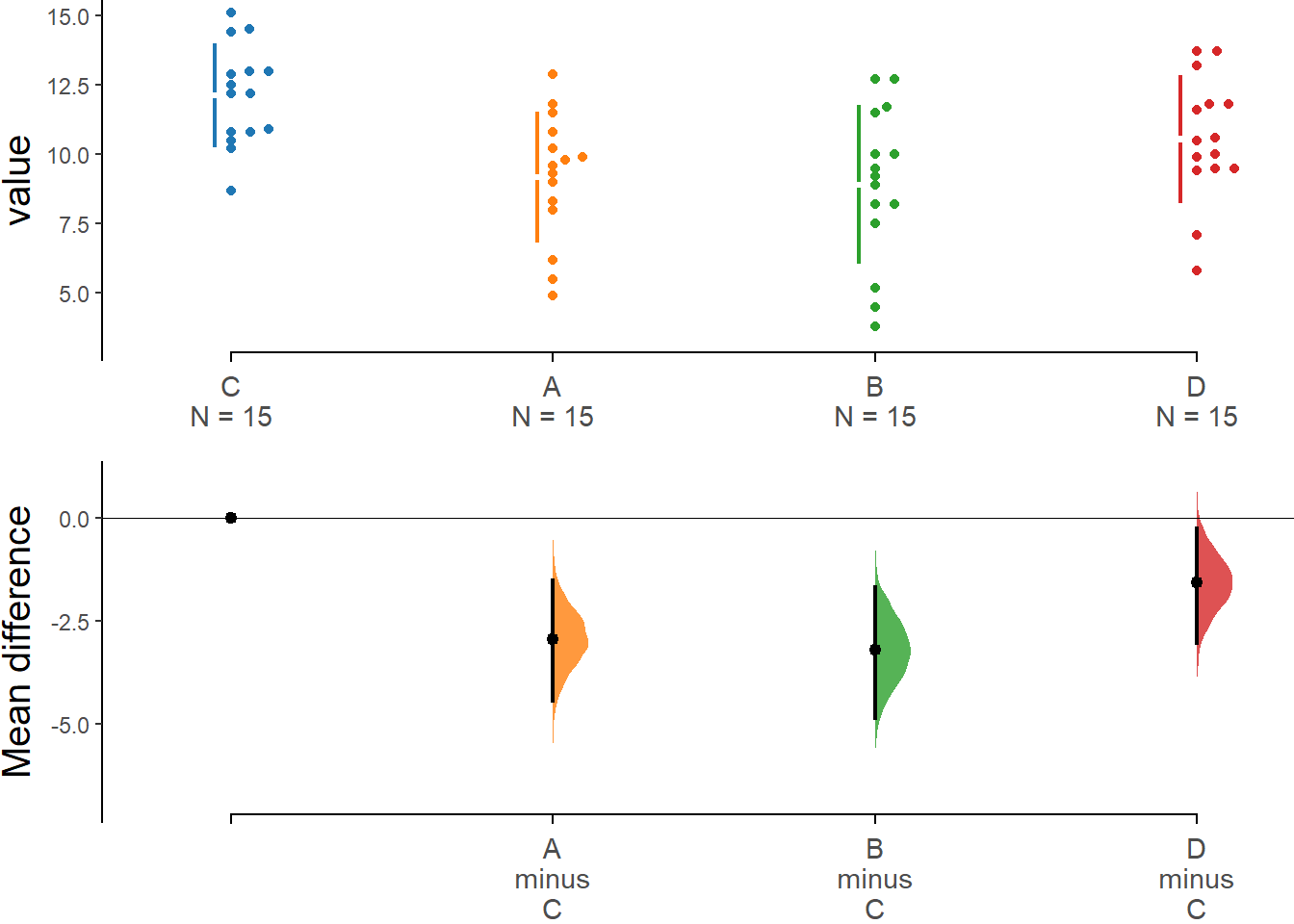

Alternatively, we can perform pairwise comparisons using pairwise t-test with the assumption of equal variances (pool.sd = TRUE) and calculate the adjusted p-values using Bonferroni correction:

pwc_Bonferroni <- dataDWL %>% 
  pairwise_t_test(
    WeightLoss ~ Diet, pool.sd = TRUE,
    p.adjust.method = "bonferroni"
    )
pwc_Bonferroni

# A tibble: 6 × 9
  .y.        group1 group2    n1    n2        p p.signif   p.adj p.adj.signif
* <chr>      <chr>  <chr>  <int> <int>    <dbl> <chr>      <dbl> <chr>       
1 WeightLoss A      B         15    15 0.746    ns       1       ns          
2 WeightLoss A      C         15    15 0.000954 ***      0.00572 **          
3 WeightLoss B      C         15    15 0.000344 ***      0.00206 **          
4 WeightLoss A      D         15    15 0.111    ns       0.669   ns          
5 WeightLoss B      D         15    15 0.0571   ns       0.343   ns          
6 WeightLoss C      D         15    15 0.0666   ns       0.399   ns

Pairwise comparisons were carried out using the method of Tukey (or Bonferroni) and the adjusted p-values were calculated.

The results in Tukey post hoc table show that the weight loss from diet C seems to be significantly larger than diet A (mean difference = 2.91 kg, 95%CI [0.71, 5.16], p=0.005 <0.05) and diet B (mean difference = 3.21 kg, 95%CI [0.98, 5.43], p=0.002 <0.05).

24.7 Welch one-way ANOVA

If the variance is different between the groups (unequal variances) then the degrees of freedom associated with the ANOVA test are calculated differently (Welch one-way ANOVA).

# Welch one-way ANOVA test (not assuming equal variance)

dataDWL %>% 
  welch_anova_test(WeightLoss ~ Diet)

# A tibble: 1 × 7
  .y.            n statistic   DFn   DFd        p method     
* <chr>      <int>     <dbl> <dbl> <dbl>    <dbl> <chr>      
1 WeightLoss    60      7.02     3  30.8 0.000989 Welch ANOVA

In this case, the Games-Howell post hoc test (or pairwise t-tests with no assumption of equal variances with Bonferroni correction) can be used to compare all possible combinations of group differences.

Games-Howell post hoc test

# Pairwise comparisons (Games-Howell)

pwc_GH <- dataDWL %>% 
  games_howell_test(WeightLoss ~ Diet)

pwc_GH

# A tibble: 6 × 8
  .y.        group1 group2 estimate conf.low conf.high p.adj p.adj.signif
* <chr>      <chr>  <chr>     <dbl>    <dbl>     <dbl> <dbl> <chr>       
1 WeightLoss A      B        -0.273   -2.82      2.28  0.991 ns          
2 WeightLoss A      C         2.93     0.872     4.99  0.003 **          
3 WeightLoss A      D         1.36    -0.898     3.62  0.371 ns          
4 WeightLoss B      C         3.21     0.849     5.56  0.005 **          
5 WeightLoss B      D         1.63    -0.889     4.16  0.308 ns          
6 WeightLoss C      D        -1.57    -3.60      0.452 0.17  ns