sem <- 240 / sqrt(64)
sem
[1] 30In statistics, a population refers to a theoretical concept representing the complete collection of individuals (which may not necessarily be people) sharing specific defining characteristics. Examples are the population of all patients with diabetes mellitus, all people with depression, or the population of all middle-aged women.
Researchers are particularly interested in quantities such as the population mean and population variance of random variables (characteristics) within these populations. These values are typically not directly observable and are denoted as parameters in statistical analysis. We use Greek lowercase letters for parameters, such as
In practice, researchers encounter constraints in resources and time, particularly when dealing with large or inaccessible populations, making it impractical to study each individual within the population (e.g., every individual with depression in the world). As a result, obtaining an exact value of a population parameter is typically unattainable. Instead, researchers analyze a sample, a subset of the population intended to be representative. In such cases, a point estimator is utilized to calculate an estimate of the unknown parameter based on the measurements obtained from the sample. For example, a sample statistic such as the sample mean can serve as an estimator for the population mean.
In most cases, the best way to get a sample that accurately represents the population is by taking a random sample from the population. When selecting a random sample, each individual in the population has equal and independent chance of being included in the sample.
The statistical framework in Figure 17.1 illustrates the process of inferring population parameters using sample statistics.
Point estimation
Point estimation is a statistical method used to estimate an unknown parameter of a population based on data collected from a sample. The objective of point estimation is to find a single, best guess or estimate for the value of the parameter. Common point estimators include the sample mean for the population mean and sample variance for the population variance.
The difference between the point estimate and the population parameter is referred to as the error in the estimate. This error constitutes a “total” error, comprised of two components:
Bias: This refers to a tendency to overestimate or underestimate the true value of the population parameter. There are numerous sources of bias in a study, including measurement bias (i.e., errors in measuring exposure or disease), sampling bias (i.e., some members of a population are systematically more likely to be selected in a sample than others), recall bias (i.e., when participants in a research study do not accurately remember a past event or experience), and attrition bias (i.e., systematic differences between study groups in the number and the way participants are lost from a study). Bias can be minimized through thoughtful design of the study (i.e., a comprehensive protocol), careful data collection procedures, and the application of suitable statistical techniques (Brown et al. 2024).
Sampling error: This measures the extent to which an estimate tends to vary from one sample to another due to random chance. Our objective is frequently to quantify and understand this variability in estimates. Standard error and confidence intervals, common measures of sampling error, are primarily influenced by both the sample size and the variability of the estimated characteristic.
Suppose a hospital is interested in finding out the average blood pressure (BP) of its diabetic patients, but measuring each patient is impractical. Instead, they randomly selected n patients from this group and measured their BP. The resulting average BP for this sample, let’s say
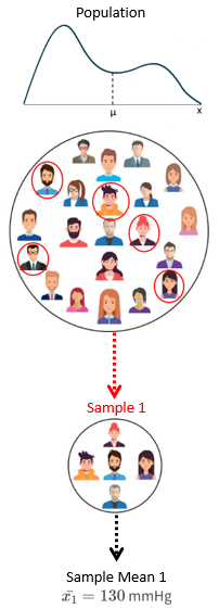
Consider repeating the sampling process by randomly selecting various samples, each consisting of n patients, and calculating their average blood pressure. This would yield a range of different sample means, such as
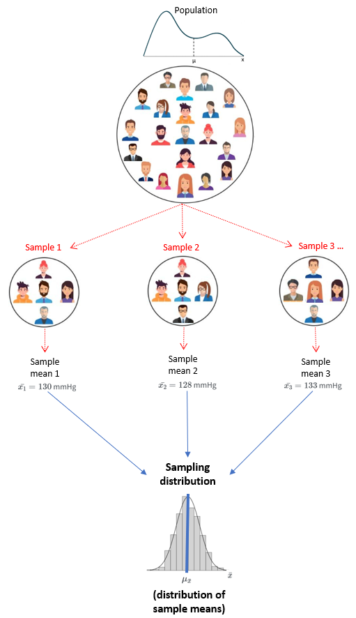
The sampling distribution is a theoretical probability distribution that represents the possible values of a sample statistic, such as the sample mean, obtained from all possible samples of a specific size drawn from a population.
| Parameter | Population | Sample | Sampling distribution of mean |
|---|---|---|---|
| Mean | |||
| Standard deviation |
The standard deviation of the sampling distribution is known as the standard error (SE). There are multiple formulas for standard error depending on what is our sampling distribution. For example, the standard error of the mean (SEM) is the population σ divided by the square root of the sample size n:
However, we usually do not know the population parameter σ; therefore, we use the sample standard deviation s, as it is an estimator of the population standard deviation.
The Standard Error of the mean (SEM) is a metric that describes the variability of sample means within the sampling distribution. In practice, it provides insight into the uncertainty associated with estimating the population mean when working with a sample, particularly when the sample size is small.
Example
The CD4 count of a sample of 64 healthy individuals has a mean of 850
The SEM provides a measure of the precision of our estimate of the population mean CD4 counts. If we were to repeat the sampling process numerous times and calculate the mean CD4 count each time, we would expect the calculated means to vary around the population mean by approximately 30
In R:
sem <- 240 / sqrt(64)
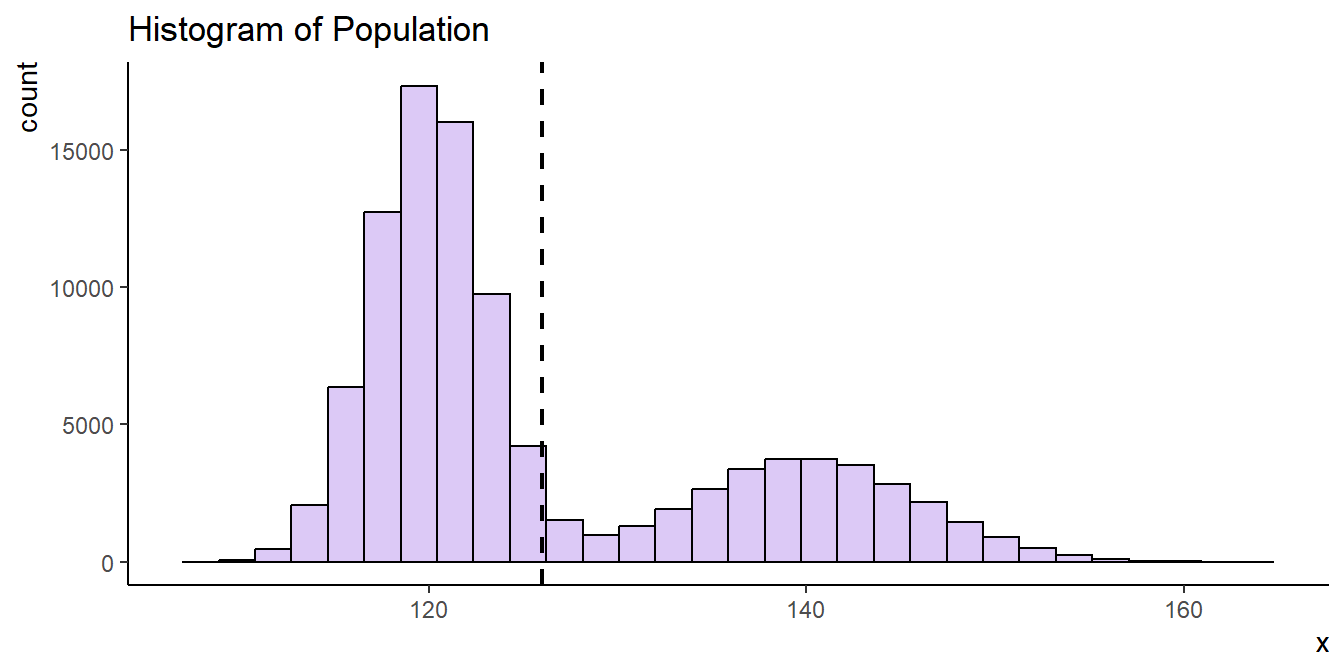
sem[1] 30Consider a population of 100,000 adults, characterized by a mean blood pressure (BP) of μ = 126 mmHg and a standard deviation of σ = 10. Now, imagine that the distribution of their BP reveals an intriguing bimodal pattern, as visually depicted in Figure 17.4.
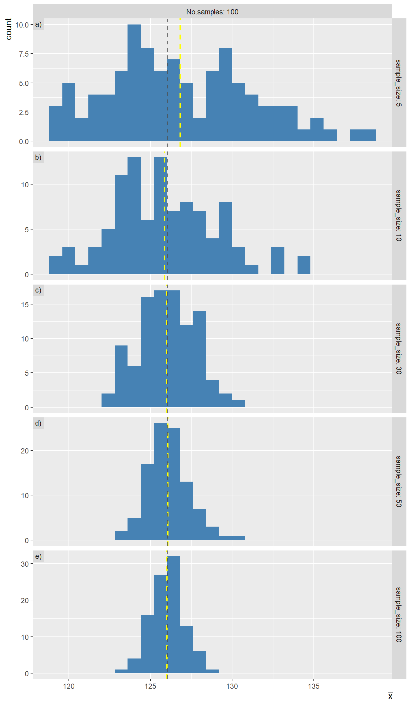
Let’s consider sampling five individuals from the population and calculating their sample mean BP, denoted as
From Figure 17.5, it is evident that as the sample size increases, the distribution of sample means tends to approximate a normal distribution, with the mean of this distribution,
Properties of the distribution of sample means
The Central Limit Theorem (CLM) for sample means in statistics states that, given a sufficiently large sample size, the sampling distribution of the mean for a variable will approximate a normal distribution regardless of the variable’s underlying distribution of the population observations:
NOTE: The CLM can be applied in inferential statistics for various test statistics, such as difference in means, difference in proportions, and the slope of a linear regression model, under the assumption of large samples and the absence of extreme skewness.
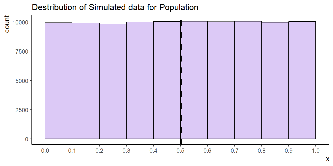
To illustrate this, let’s generate some data from a continuous uniform distribution (100,000 observations):
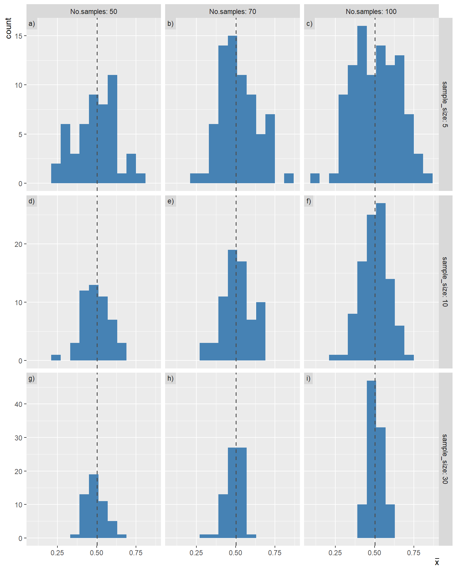
We can consider the data we’ve just created above as the entire population (N=100,000) from which we can sample. We sample a bunch of times with different number of samples (50, 70, 100) and simple sizes (5, 10, 30) and we generate the histograms of the sample means (Figure 17.7).
We observe that the distribution of sample means for sample size of five exhibits considerable variability (Figure 17.7 a, b, c). As we take a large number of sample means and the sample size is increased to 30, the distributions become increasingly symmetric, with less variability, and tend toward approximate normality (Figure 17.7 f, i).