28  Correlation

Correlation is a statistical method used to assess a possible association between two numeric variables, X and Y. There are several statistical coefficients that we can use to quantify correlation depending on the underlying relation of the data. In this chapter, we’ll learn about four correlation coefficients:

• Pearson’s \(r\)
• Spearman’s \(r_{s}\) and and Kendall’s \(\tau\)
• Coefficient \(ξ\)

Pearson’s coefficient measures linear correlation, while the Spearman’s and Kendall’s coefficients compare the ranks of data and measure monotonic associations. The new \(ξ\) correlation coefficient is more appropriate to measure the strength of non-monotonic associations.

When we have finished this Chapter, we should be able to:

Learning objectives

• Explain the concept of correlation of two numeric variables.
• Understand the most commonly used correlation coefficients: Pearson’s r, Spearman’s \(r_{s}\), and the new \(ξ\) coefficient.
• Discuss the possible meaning of correlation that we observe.

28.1 Research question

We consider the data in Birthweight dataset. Let’s say that we want to explore the association between weight (in g) and height (in cm) for a sample of 550 infants of 1 month age.

28.2 Packages we need

We need to load the following packages:

library(rstatix)
library(XICOR)
library(ggExtra)
library(patchwork)
library(here)
library(tidyverse)
library(gt)
library(report)

28.3 Preparing the data

We import the data BirthWeight in R:

library(readxl)
BirthWeight <- read_excel(here("data", "BirthWeight.xlsx"))

Figure 28.1: Table with data from “BirthWeight” file.

We inspect the data and the type of variables:

glimpse(BirthWeight)

Rows: 550
Columns: 6
$ weight    <dbl> 3950, 4630, 4750, 3920, 4560, 3640, 3550, 4530, 4970, 3740, …
$ height    <dbl> 55.5, 57.0, 56.0, 56.0, 55.0, 51.5, 56.0, 57.0, 58.5, 52.0, …
$ headc     <dbl> 37.5, 38.5, 38.5, 39.0, 39.5, 34.5, 38.0, 39.7, 39.0, 38.0, …
$ gender    <chr> "Female", "Female", "Male", "Male", "Male", "Female", "Femal…
$ education <chr> "tertiary", "tertiary", "year12", "tertiary", "year10", "ter…
$ parity    <chr> "2 or more siblings", "Singleton", "2 or more siblings", "On…

The data set BirthWeight has 550 infants of 1 month age (rows) and includes six variables (columns). Both the weight and height are numeric (<dbl>) variables.

28.4 Plot the data

A first step that is usually useful in studying the association between two numeric variables is to prepare a scatter plot of the data. The pattern made by the points plotted on the scatter plot usually suggests the basic nature and strength of the association between two variables.

p <- ggplot(BirthWeight, aes(height, weight)) +
  geom_point(color = "blue", size = 2) +
  theme_minimal(base_size = 14)

ggMarginal(p, type = "histogram", 
           xparams = list(fill = 7),
           yparams = list(fill = 3))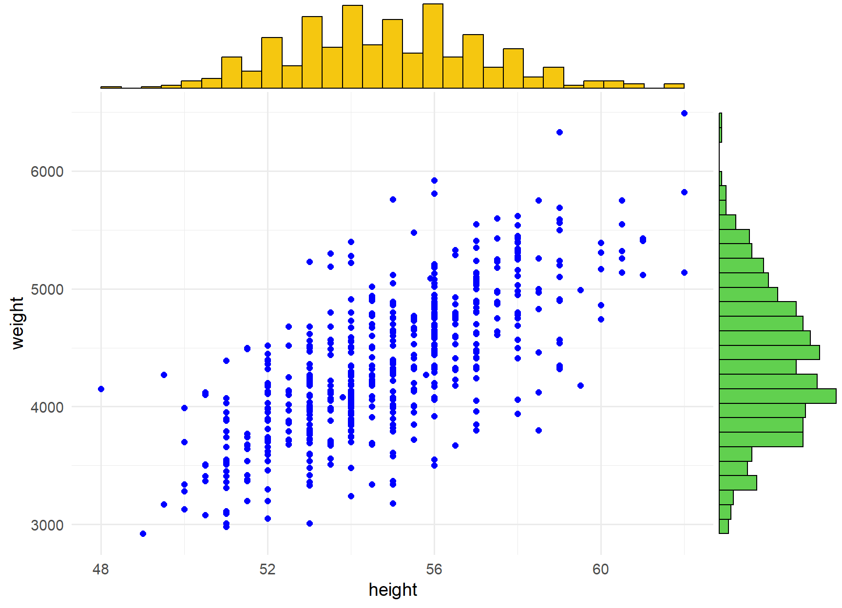

Figure 28.2: Scatter plot of the association between height and weight in 550 infants of 1 month age.

28.5 Linear correlation (Pearson’s coefficient \(r\))

28.5.1 The formula

Given a set of \({n}\) pairs of observations \((x_{1},y_{1}),\ldots ,(x_{n},y_{n})\) with means \(\bar{x}\) and \(\bar{y}\) respectively, \(r\) is defined as:

\[r = \frac{\sum_{i=1}^n (x_i - \bar{x})(y_i - \bar{y})}{\sqrt{\sum_{i=1}^n (x_i - \bar{x})^2 \sum_{i=1}^n(y_i - \bar{y})^2}} \tag{28.1}\]

We observe that the Equation 28.1 is based on calculating the sum of the product \((x_i - \bar{x})(y_i - \bar{y})\). In our example, that is the the sum of the product \((height_{i} - \overline{height}) \cdot (weight_{i} - \overline{weight})\). Our approach begins by examining the signs of these products.

 

Figure 28.3: Scatter plot with two pink axes intersecting at the mean point of the variables. The vertical distances of the data points from these axes express the deviations from the mean.

 

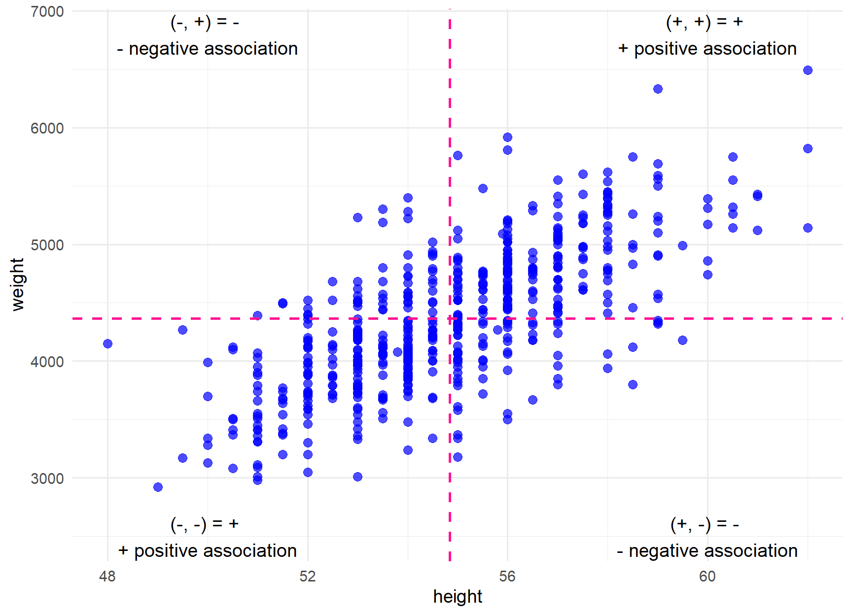
Positive product: In the top-right pane of the Figure 28.3, the deviations from the mean for both variables, height and weight, are positive. Consequently, their products will also be positive. In the bottom-left pane, the deviations from the mean for both variables are negative. Once again, their product will be positive.

Negative product: In the top-left pane of the Figure 28.3, the deviation of height from its mean is negative, while the deviation of weight is positive. Therefore, their product will be negative. Similarly, in the bottom-right pane, the product will be negative.

We observe that most of the products are positive. By applying the Equation 28.1, we can calculate the Pearson’s correlation coefficient, a task that can be easily carried out using R:

cor(BirthWeight$height, BirthWeight$weight)

[1] 0.7131192

Characteristics of Pearson’s correlation coefficient \(r\)

The \(r\) statistic shows the direction and measures the strength of the linear association between the variables. It is a dimensionless quantity that takes a value in the range -1 to +1.

Direction of the association

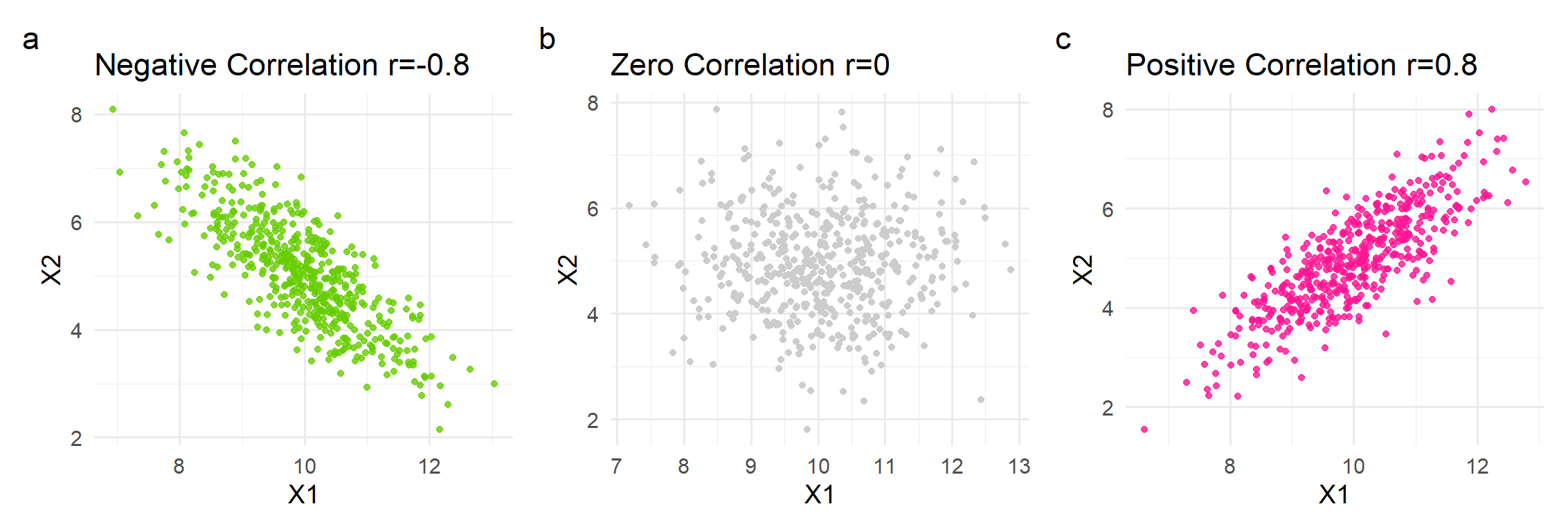
A negative correlation coefficient indicates that as one variable increases, the other variable tends to decrease, and vice versa (Figure 28.4 a). A zero value indicates that no association exists between the two variables (Figure 28.4 b). A positive coefficient indicates that both variables increase (or decrease) together (Figure 28.4 c).

Figure 28.4: The direction of association can be (a) negative, (b) no association, or (c) positive.

 

Strength of the association

The strength of the association range from -1 to +1. The stronger the correlation, the more closely the correlation coefficient approaches ±1. A correlation coefficient of -1 or +1 indicates a perfect negative or positive association, respectively (Figure 28.5 c and f).

Figure 28.5: The stronger the correlation, the more closely the correlation coefficient approaches ±1.

 

The Table 28.1 demonstrates how to interpret the strength of an association according to (Evans 1996).

Table 28.1: Interpretation of the values of the sample estimate of the correlation coefficient.

Value of r	Strength of association
\(|r| \geq{0.8}\)	very strong association
\(0.6\leq|r| < 0.8\)	strong association
\(0.4\leq|r| < 0.6\)	moderate association
\(0.2\leq|r| < 0.4\)	weak association
\(|r| < 0.2\)	very weak association

In our example, the coefficient equals r = 0.713, indicating that infants with greater height generally exhibit higher weight. We say that there is a linear positive association between the two variables. However, correlation does not mean causation (Altman and Krzywinski 2015).

Even though summary statistics, such as Pearson r, can provide useful information, they are just simplified representations of the data and may not always capture the full picture. This is typically demonstrated with the Anscombe’s quartet, highlighting the need to explore and understand the underlying patterns and associations within the data through graphical representations (Figure 28.6).

Anscombe’s Quartet

Anscombe’s quartet consists of four sets of data, each containing eleven (x, y) points. Despite having the same basic statistical characteristics, these datasets exhibit distinct distributions and present remarkable differences in their graphical representations (Anscombe 1973).

Figure 28.6: Anscombe’s quartet. All datasets have a Pearson’s correlation of r = 0.82.

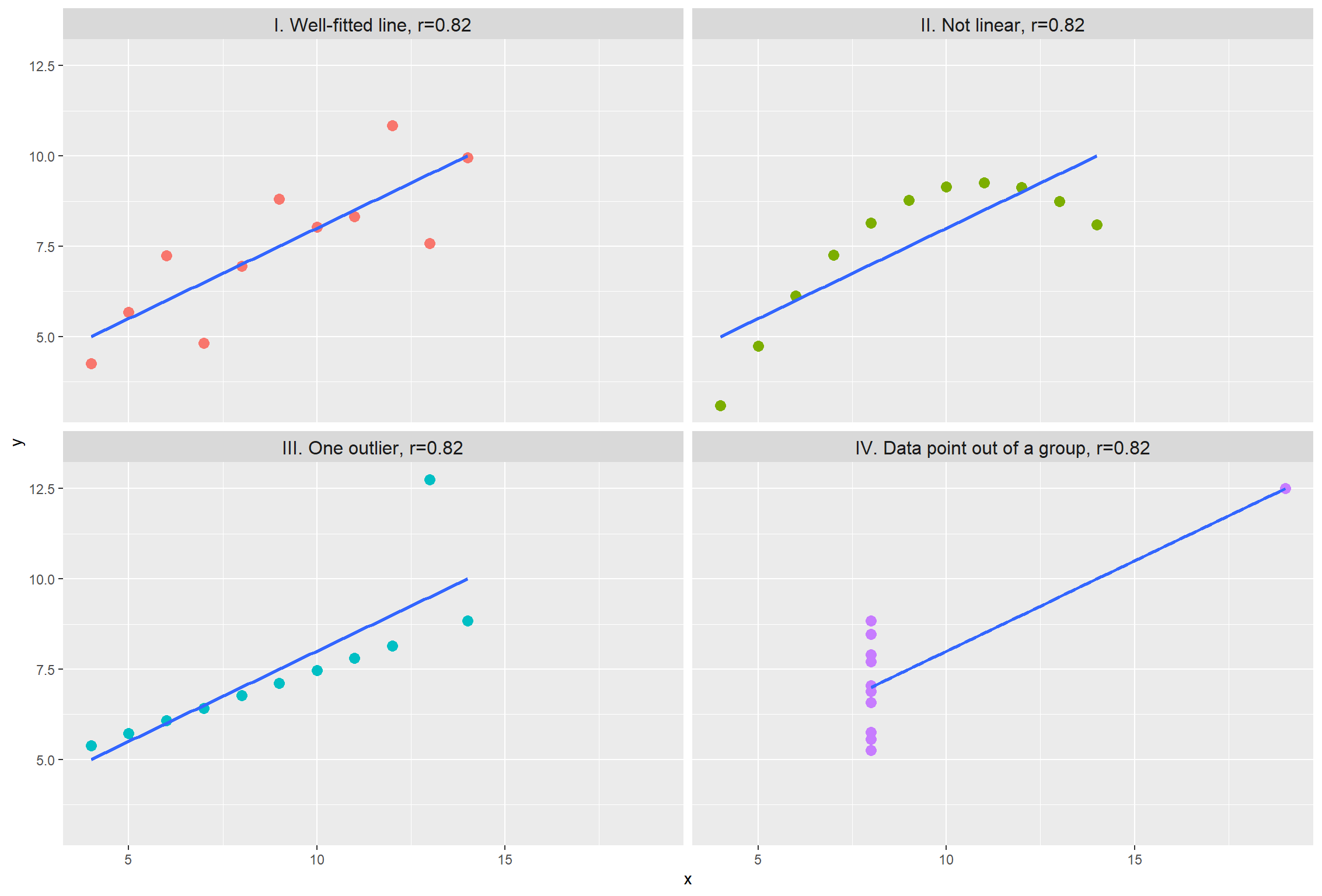
Even though all datasets have a Pearson’s correlation equal to 0.82, their graphical representations are very different. Figure 28.6 I depicts a linear association where the application of Pearson’s correlation would be appropriate. Figure 28.6 II shows a non-linear association and a non-parametric analysis would be appropriate. Figure 28.6 III demonstrates a nearly perfect linear association (approaching r = 1), but the presence of an outlier has caused a reduction in the correlation coefficient. Figure 28.6 IV shows no association between the two variables (X, Y), although an outlier has artificially increased the correlation value.

 

28.5.2 Hypothesis Testing

Null hypothesis and alternative hypothesis

• \(H_0\): There is no linear association between the two numeric variables (they are independent, \(ρ = 0\))
• \(H_1\): There is linear association between the two numeric variables (they are dependent, \(ρ \neq 0\))

28.5.3 Assumptions

Before we conduct a statistical test for the Pearson r coefficient, we should make sure that some assumptions are met.

Check if the following assumptions are satisfied

1. The variables are observed on a random sample of individuals (each individual should have a pair of values).
   
2. There is a linear association between the two variables. If the association is nonlinear, the correlation coefficient might not accurately represent the association between the variables.
3. For a valid hypothesis testing and calculation of confidence intervals both variables should have an approximately normal distribution.
4. Absence of outliers in the data set. It’s important to identify and address outliers before calculating the coefficient.

Based on the Figure 28.2 the points seem to be scattered around an invisible line without any important outlier value. Additionally, the marginal histograms show that the data are approximately normally distributed (we have a large sample so the graphs are reliable) for both weight and height. Therefore, we conclude that the assumptions are satisfied.

28.5.4 Run the test

To determine whether to reject the null hypothesis or not, a test is conducted based on the formula:

\[t = \frac{r}{SE_{r}}=\frac{r}{\sqrt{(1-r^2)/(n-2)}} \tag{28.2}\]

where n is the sample size.

For the data in our example, the number of observations are n= 550, r= 0.713 and \(SE_{r}=\sqrt{ \frac{(1-0.713^2)}{(550-2)}}= \sqrt{ \frac{(1-0.5084)}{548}} = \sqrt{\frac{0.4916}{548}}= 0.0299\).

According to Equation 29.17:

\[t = \frac{r}{SE_{r}}= \frac{0.713}{0.0299}= 23.8\]

In this example, the value for the test statistic equals 23.8. Using R, we can find the 95% confidence interval and the corresponding p-value for a two tailed test:

Pearson’s correlation test

Base R

cor.test(BirthWeight$height, BirthWeight$weight) # the default method is "pearson"

    Pearson's product-moment correlation

data:  BirthWeight$height and BirthWeight$weight
t = 23.813, df = 548, p-value < 2.2e-16
alternative hypothesis: true correlation is not equal to 0
95 percent confidence interval:
 0.6694248 0.7518965
sample estimates:
      cor 
0.7131192 

rstatix

BirthWeight |> 
  cor_test(height, weight)   # the default method is "pearson"  

# A tibble: 1 × 8
  var1   var2     cor statistic        p conf.low conf.high method 
  <chr>  <chr>  <dbl>     <dbl>    <dbl>    <dbl>     <dbl> <chr>  
1 height weight  0.71      23.8 1.40e-86    0.669     0.752 Pearson

The result is significant (p < 0.001) and we reject the null hypothesis.

Important

The significance of correlation is influenced by the size of the sample. With a large sample size, even a weak association may be significant, whereas with a small sample size, even a strong association might or might not be significant.

28.5.5 Present the results

Summary table

BirthWeight |> 
  cor_test(height, weight) |>
  gt() |> 
  fmt_number(columns = starts_with(c("c", "st", "p")), 
             decimals = 3)

var1	var2	cor	statistic	p	conf.low	conf.high	method
height	weight	0.710	23.813	0.000	0.669	0.752	Pearson

Report the results (according to Evans 1996)

cor.test(BirthWeight$height, BirthWeight$weight) |> 
  report(rules = "evans")

Effect sizes were labelled following Evans's (1996) recommendations.

The Pearson's product-moment correlation between BirthWeight$height and
BirthWeight$weight is positive, statistically significant, and strong (r =
0.71, 95% CI [0.67, 0.75], t(548) = 23.81, p < .001)

  We can use the above information to write up a final report:

Final report

We observed a strong, positive linear association between height and weight of one-month-old infants which is significant (Pearson r = 0.71, 95% CI [0.67, 0.75], n = 550, p < 0.001).

 

28.6 Rank correlation (Spearman’s \(r_{s}\) and Kendall’s \(\tau\) coefficients)

Spearman’s correlation \(r_{s}\) and Kendall’s coefficient \(\tau\) are both non-parametric correlation coefficients used to measure the strength and direction of association between two variables. Both coefficients are based on the concept of ranking the data but they employ distinct methods in their calculation and have some different characteristics (Puth, Neuhäuser, and Ruxton 2015).

Characteristics of Spearman’s and Kendall’s coefficients

The range of both coefficients is between −1 and 1 and the interpretation of rank correlation coefficients is similar to the Pearson’s correlation coefficient. However, the focus is on assessing the monotonic association between variables, rather than just the linear association.

In a monotonic association the variables tend to move in the same relative direction, but not necessarily at a constant rate. Note that while all linear associations can be considered monotonic (Figure 28.7 a), the reverse isn’t always true, as monotonic associations can also take on non-linear forms (Figure 28.7 b).

Figure 28.7: The association can be (a) linear monotonic and (b) monotonic non-linear.

 

28.6.1 Hypothesis Testing

Null hypothesis and alternative hypothesis

• \(H_0\): There is no monotonic association between the two numeric variables (they are independent)
• \(H_1\): There is monotonic association between the two numeric variables (they are dependent)

28.6.2 Assumptions

Check if the following assumptions are satisfied

1. The variables are observed on a random sample of individuals (each individual should have a pair of values).
2. There is a monotonic association between the two variables.

28.6.3 Run the test

Spearman’s correlation test

Base R

cor.test(BirthWeight$height, BirthWeight$weight, method = "spearman")

Warning in cor.test.default(BirthWeight$height, BirthWeight$weight, method =
"spearman"): Cannot compute exact p-value with ties

    Spearman's rank correlation rho

data:  BirthWeight$height and BirthWeight$weight
S = 8013119, p-value < 2.2e-16
alternative hypothesis: true rho is not equal to 0
sample estimates:
     rho 
0.711021 

rstatix

BirthWeight |> 
  cor_test(height, weight, method = "spearman")  

# A tibble: 1 × 6
  var1   var2     cor statistic       p method  
  <chr>  <chr>  <dbl>     <dbl>   <dbl> <chr>   
1 height weight  0.71  8013119. 7.4e-86 Spearman

Kendall’s correlation test

Base R

cor.test(BirthWeight$height, BirthWeight$weight, method = "kendall")

    Kendall's rank correlation tau

data:  BirthWeight$height and BirthWeight$weight
z = 18.359, p-value < 2.2e-16
alternative hypothesis: true tau is not equal to 0
sample estimates:
      tau 
0.5408389 

rstatix

BirthWeight |> 
  cor_test(height, weight, method = "kendall")  

# A tibble: 1 × 6
  var1   var2     cor statistic        p method 
  <chr>  <chr>  <dbl>     <dbl>    <dbl> <chr>  
1 height weight  0.54      18.4 2.78e-75 Kendall

 

We observe that Kendall’s \(\tau\) is smaller than Spearman’s \(r_s\) correlation (0.54 vs 0.71).

28.6.4 Present the results for Spearman’s correlation test

Summary table

BirthWeight |> 
  cor_test(height, weight, method = "spearman") |>
  gt() |> 
  fmt_number(columns = starts_with(c("c", "p")),
             decimals = 3)

var1	var2	cor	statistic	p	method
height	weight	0.710	8013119	0.000	Spearman

Report the results (according to Evans 1996)

cor.test(BirthWeight$height, BirthWeight$weight, method = "spearman") |> 
report(rules = "evans")

Warning in cor.test.default(BirthWeight$height, BirthWeight$weight, method =
"spearman"): Cannot compute exact p-value with ties

Effect sizes were labelled following Evans's (1996) recommendations.

The Spearman's rank correlation rho between BirthWeight$height and
BirthWeight$weight is positive, statistically significant, and strong (rho =
0.71, S = 8.01e+06, p < .001)

  We can use the above information to write up a final report:

Final report

We observed a strong, positive monotonic association between height and weight of one-month-old infants which is significant (Spearman \(r_s\) = 0.71, n = 550, p < 0.001).

 

28.6.5 Present the results for Kendall’s correlation test

Summary table

BirthWeight |> 
  cor_test(height, weight, method = "kendall") |>
  gt() |> 
  fmt_number(columns = starts_with(c("c", "st", "p")),
             decimals = 3)

var1	var2	cor	statistic	p	method
height	weight	0.540	18.359	0.000	Kendall

Report the results (according to Evans 1996)

cor.test(BirthWeight$height, BirthWeight$weight, method = "kendall") |> 
report(rules = "evans")

Effect sizes were labelled following Evans's (1996) recommendations.

The Kendall's rank correlation tau between BirthWeight$height and
BirthWeight$weight is positive, statistically significant, and moderate (tau =
0.54, z = 18.36, p < .001)

  We can use the above information to write up a final report:

Final report

We observed a moderate, positive monotonic association between height and weight of one-month-old infants which is significant (Kendall \(\tau\) = 0.54, n = 550, p < 0.001).

 

28.7 Non-monotonic association (coefficient \(ξ\))

The correlation coefficient \(ξ\) ranges from 0 to 1 and is a measure of dependence between X and Y variables (Chatterjee 2021). It equals 1 when the Y is a function of X and it equals 0 when X and Y are independent. Thus, \(ξ\) gives a measure of the strength of the association and it can be used for non-monotonic associations. However, for monotonic associations, it does not indicate the direction of the association.

28.7.1 Hypothesis Testing

Null hypothesis and alternative hypothesis

• \(H_0\): There is not association between the two numeric variables (they are independent)
• \(H_1\): There is association between the two numeric variables (they are dependent)

28.7.2 Assumptions

Check if the following assumptions are satisfied

1. The variables are observed on a random sample of individuals (each individual should have a pair of values).

28.7.3 Run the test

xicor(BirthWeight$height, BirthWeight$weight, pvalue = TRUE)

$xi
[1] 0.3163988

$sd
[1] 0.02697177

$pval
[1] 0

28.7.4 Present the results

Based on the \(ξ\) correlation coefficient, there is a significant association between height and weight (\(ξ\) = 0.31, sd = 0.027, p < 0.001).

 

NOTE

In our example, there is a linear association between the height and weight, so the most appropriate correlation measure is the Pearson’s coefficient. Now, consider another example with a non-monotonic association between X and Y, as illustrated in Figure 28.8:

Figure 28.8: Non-monotonic association.

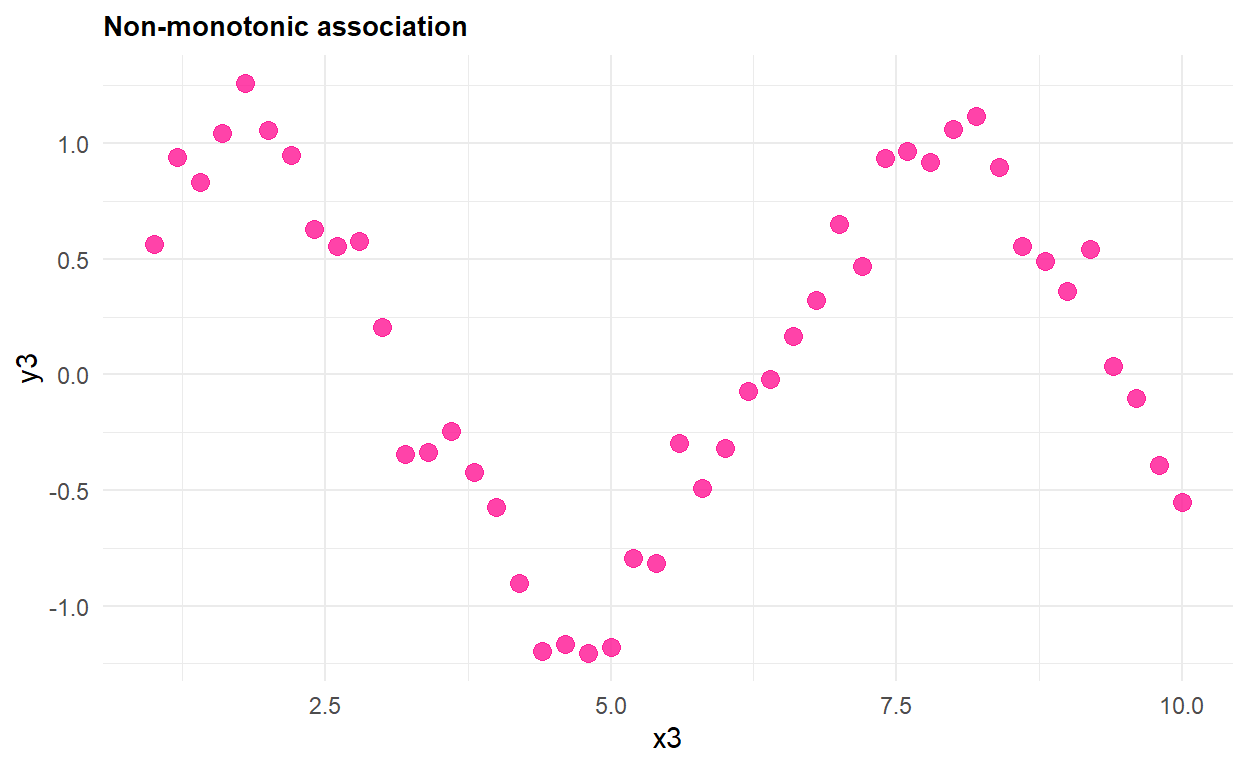
Let’s calculate in R the correlation coefficients for this data set:

cor(df3$x3, df3$y3)

[1] -0.04640522

cor(df3$x3, df3$y3, method = "spearman")

[1] -0.08800493

cor(df3$x3, df3$y3, method =  "kendall")

[1] -0.047343

xicor(df3$x3, df3$y3)

[1] 0.7021277

In this case, the correlation coefficient that is appropriate to be used is the \(ξ\) correlation coefficient.

Altman, Naomi, and Martin Krzywinski. 2015. “Association, Correlation and Causation.” Nature Methods 12 (10): 899–900. https://doi.org/10.1038/nmeth.3587.

Anscombe, F. J. 1973. “Graphs in Statistical Analysis.” The American Statistician 27 (1): 17. https://doi.org/10.2307/2682899.

Chatterjee, Sourav. 2021. “A New Coefficient of Correlation.” Journal of the American Statistical Association 116 (536): 2009–22. https://doi.org/10.1080/01621459.2020.1758115.

Evans, James D. 1996. Straightforward Statistics for the Behavioral Sciences. Straightforward Statistics for the Behavioral Sciences. Belmont, CA, US: Thomson Brooks/Cole Publishing Co.

Puth, Marie-Therese, Markus Neuhäuser, and Graeme D. Ruxton. 2015. “Effective Use of Spearman’s and Kendall’s Correlation Coefficients for Association Between Two Measured Traits.” Animal Behaviour 102 (April): 77–84. https://doi.org/10.1016/j.anbehav.2015.01.010.