n <- 20
mu <- 0.75
x_bar <- 0.96
s <- 0.35


se <- s/sqrt(n)
t <- (x_bar-mu)/se
t
[1] 2.683282Hypothesis testing is a widely used method in research to make inferences about population parameters based on sample data. In the context of health sciences, it is often used to evaluate the effectiveness of interventions, compare treatment outcomes, assess the significance of risk factors, and investigate various health-related phenomena.
Hypothesis testing is a statistical method used to assess whether the data are consistent with the null hypothesis (
Step 1: State the null hypothesis,
NOTE: We decide a non-directional
Step 2: Set a level of significance, α (usually 0.05).
Step 3: Determine an appropriate statistical test, check for any assumptions that may exist, and calculate the test statistic.
NOTE: There are two basic types of statistical tests, parametric and non-parametric. Parametric tests (e.g., t-test, ANOVA), depend on assumptions about the distribution of the parameter being studied. Non-parametric tests (e.g., Mann-Whitney U test, Kruskal-Wallis test), use some way of ranking the measurements and do not require such assumptions. However, non-parametric tests are typically about 95% as powerful as parametric tests.
Step 4: Decide whether or not the result is “statistically” significant according to (a) the rejection region or (b) the p-value.
(a) The rejection region approach
Based on the known sampling distribution of the test statistic, the rejection region is a set of values for the test statistic for which the null hypothesis is rejected. If the observed test statistic falls within the rejection region, then we reject the null hypothesis.
(b) The p-value approach
The p-value is the probability of obtaining the observed results, or something more extreme, if the null hypothesis is true.
We compare the calculated p-value to the significance level α:
The Table 19.1 demonstrates how to interpret the strength of the evidence. However, always keep in mind the size of the study being considered.
| p-value | Interpretation |
|---|---|
| No evidence to reject |
|
| Weak evidence to reject |
|
| Evidence to reject |
|
| Strong evidence to reject |
|
| Very strong evidence to reject |
Step 5: Interpret the results and draw a “real world” conclusion.
NOTE: Even if a result is statistically significant, it may not be clinically significant if the effect size is small or if the findings do not have practical implications for patient care.
In the framework of hypothesis testing there are two types of errors: Type I error (False Positive) and Type II error (False Negative) (Table 19.2).
Type I error: we reject the null hypothesis when it is true (false positive), leading us to conclude that there is an effect when, in reality, there is none. The maximum chance (probability) of making a Type I error is denoted by α (alpha), which represents the significance level of the test and is typically set at 0.05 (5%); we reject the null hypothesis if our p-value is less than the significance level, i.e. if p < a.
Type II error: we do not reject the null hypothesis when it is false (false negative), and conclude that there is no effect when one really exists. The chance of making a Type II error is denoted by β (beta) and should be no more than 0.20 (20%); its compliment, (1 - β), is the power of the test.
| In population |
|||
|---|---|---|---|
| True | False | ||
|
Decision based on the sample |
Do Not Reject |
Correct decision: |
Type II error ( |
|
Reject |
Type I error ( |
Correct decision: |
The power (
| Factor | Influence on study’s power |
|---|---|
|
Effect Size (e.g., mean difference, risk ratio) |
As effect size increases, power tends to increase (a larger effect size is easier to be detected by the statistical test, leading to a greater probability of a statistically significant result). |
| Sample Size | As the sample size goes up, power generally goes up (this factor is the most easily manipulated by researchers). |
| Standard deviation | As variability decreases, power tends to increase (variability can be reduced by controlling extraneous variables such as inclusion and exclusion criteria defining the sample in a study). |
| Significance level α | As α goes up, power goes up (it would be easier to find statistical significance with a larger α, e.g. α=0.1, compared to a smaller α, e.g. α=0.05). |
Let’s explore the hypothesis testing procedure through a simple example such as the one sample t-test.
Example
Suppose the mean serum creatinine in healthy adult women is 0.75 mg/dl. A research study was conducted to examine the serum creatinine levels in female patients with diabetes. Twenty female patients were randomly enrolled, with a mean serum creatinine level of 0.96 mg/dl and a standard deviation of 0.35 mg/dl. Assuming that the serum creatinine follows a normal distribution, is the mean serum creatinine in diabetic patients significantly different from that in healthy adults, with a level of significance of
Step 1: State the null and alternative hypotheses
In our example, the null hypothesis
In our example, we adopt a two-sided hypothesis, implying that the mean serum creatinine in female patients with diabetes may differ from
Step 2: Set the level of significance, α
We set the significance level (type I error) as α = 0.05.
Step 3: Determine an appropriate statistical test, check for any assumptions that may exist, and calculate the test statistic.
We choose a t-test, a statistical method utilized to assess whether the mean of a single sample differs significantly from a known population mean. This statistical test is particularly effective when dealing with small sample sizes and when the population standard deviation is unknown. The main assumption underlying the t-test is that the data being analyzed follows a normal distribution.
The formula for the test statistic t is:
so,
In R:
n <- 20
mu <- 0.75
x_bar <- 0.96
s <- 0.35
se <- s/sqrt(n)
t <- (x_bar-mu)/se
t[1] 2.683282Step 4: Decide whether or not the result is “statistically” significant.
(a) The rejection region approach
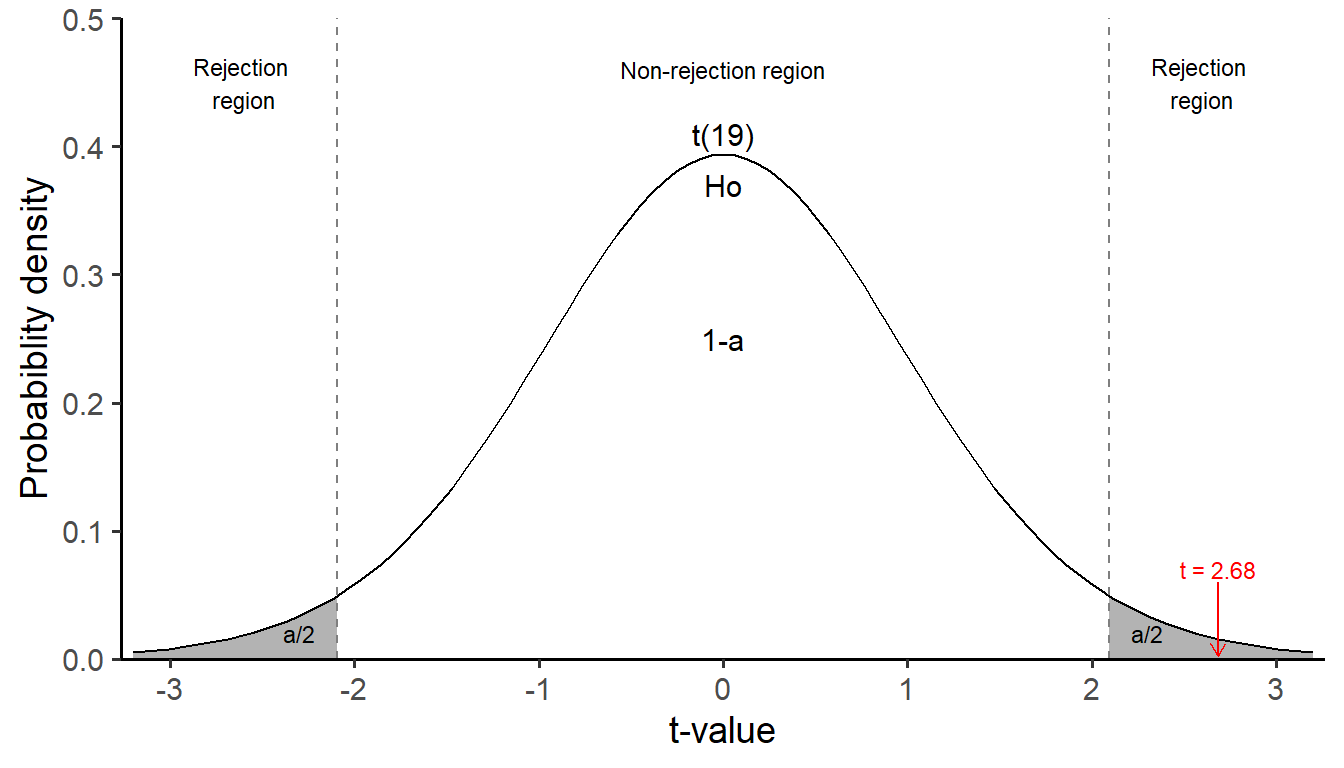
Next, we utilize the t-distribution with n-1 degrees of freedom (df = 20-1 = 19), encompassing all possible values of the test statistic t and their associated probabilities. The area under the curve is divided into one central non-rejection region and two-sided, grey rejection regions defined by the presepcified level of significance
In our example, the observed value of the test statistic, t = 2.68, falls within the upper grey rejection region, leading us to reject the null hypothesis
(b) The p-value approach
The second approach involves assigning a probability to the value of the test statistic. Particularly, if the test statistic is exceptionally extreme under the assumption that the null hypothesis holds true, it is given a low probability. Conversely, if the test statistic is less unusual, it receives a higher probability.
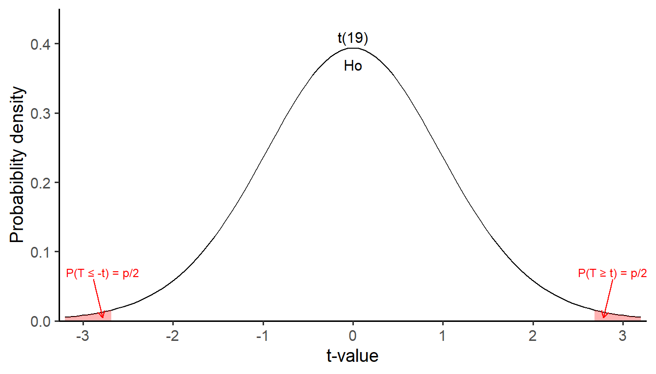
The corresponding probability for the test statistic t can be calculated by summing the two cumulative probabilities P(T ≤ -t) and P(T ≥ t). Therefore, the p-value is computed as 2*P(T ≥ t), given that we are conducting a two-tailed test and there is symmetry in the t-distribution with df = n-1 (Figure 19.2).
P <- pt(t, df = n-1, lower.tail = F)

p_value <- 2*P
p_value
[1] 0.01470991The resulting p-value is 0.0147 which is less than 0.05, so we reject the null hypothesis.
Step 5: Interpret the results and draw a “real world” conclusion.
At the 5% significance level, the test result provides evidence against the null hypothesis (p = 0.014 < 0.05). The mean serum creatinine in women with diabetes (0.96 mg/dl) is significantly higher than the serum creatinine in healthy adult women (0.75 mg/dl).
Hypothesis testing and confidence intervals are both inferential methods based on the concept of sampling distribution. Although closely related, they serve distinct purposes. Specifically, hypothesis testing involves a statistical decision (reject or not reject a pre-defined hypothesis) based on the p-value, while confidence intervals provide an interval estimate of the effect size and its associated precision.
Let’s calculate the 95% CI for the mean using the t-distribution:
where
t_star <- qt(0.025, df = n-1, lower.tail = F)

# compute lower limit of 95% CI
lower_95CI <- x_bar - t_star*se
lower_95CI

# compute upper limit of 95% CI
upper_95CI <- x_bar + t_star*se
upper_95CI
[1] 0.796195
[1] 1.123805We observe that the value of null hypothesis,
The impact of study design decisions, such as the size of the sample, on research outcomes and conclusions is a crucial aspect that researchers must carefully consider before conducting the study. Let’s return to the example provided earlier, but this time the researchers designed a study with only 10 patients (we suppose everything else is the same).
First, we calculate the new value of the t test statistic:
n <- 10
se <- s/sqrt(n)
t <- (x_bar-mu)/se
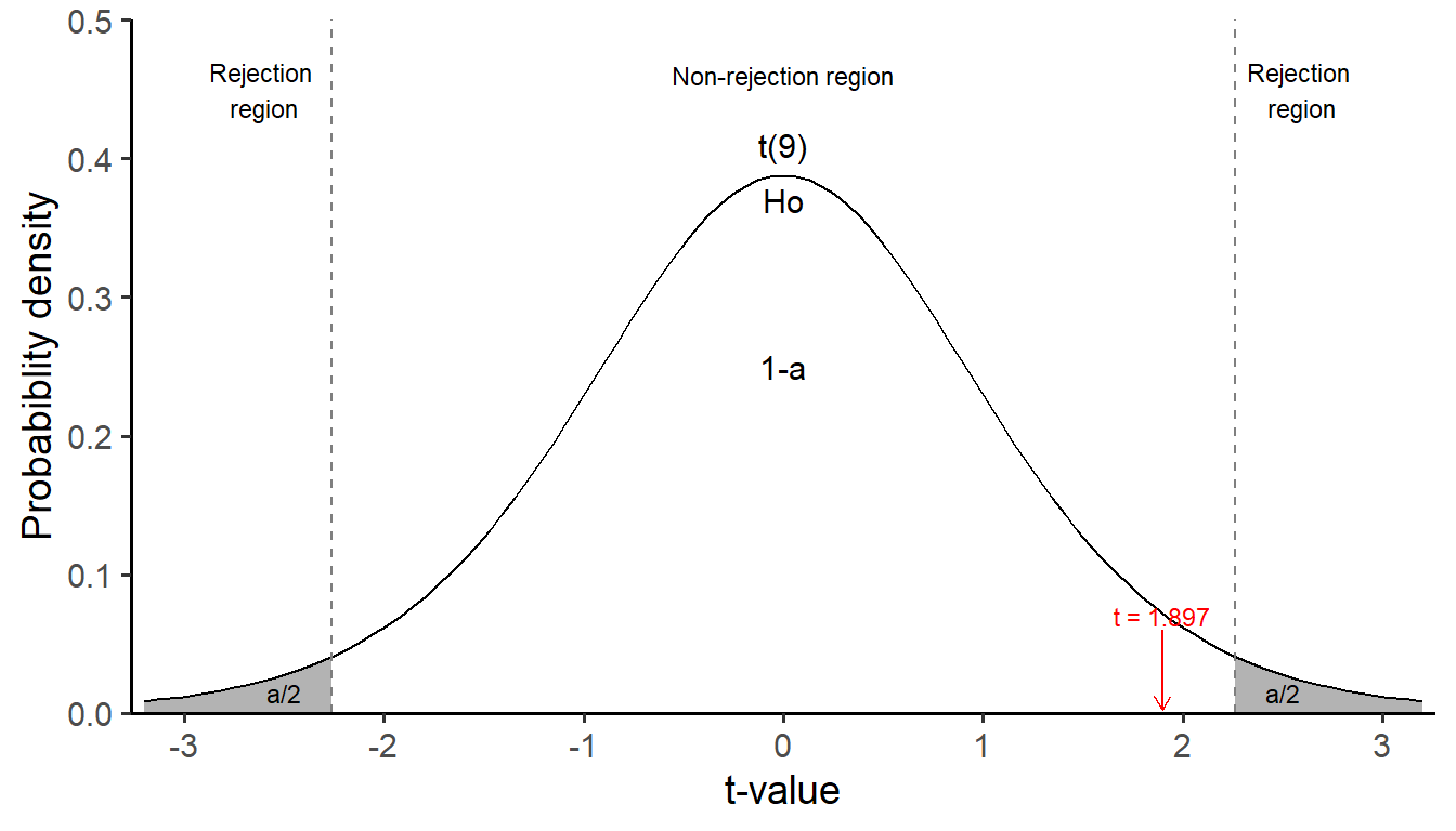
t[1] 1.897367Next, we will graphically present the two approaches, illustrating the rejection region and p-value methods.
(a) The rejection region approach
In this instance, the observed test statistic value, t = 1.897, falls within the non-rejection region, thus indicating that we do not reject the null hypothesis
(b) The p-value approach
The p-value is computed as 2*P(T ≥ t) (Figure 19.3):
P <- pt(t, df = n-1, lower.tail = F)

p_value <- 2*P
p_value
[1] 0.09026733The resulting p-value is 0.09 which is greater than
Additionally, the 95% confidence interval is following:
# compute lower limit of 95% CI
lower_95CI <- x_bar - t_star*se
lower_95CI

# compute upper limit of 95% CI
upper_95CI <- x_bar + t_star*se
upper_95CI
[1] 0.7096251
[1] 1.210375We observe that the 95% confidence interval is wider [0.709, 1.21] and includes the value of null hypothesis,
Even when a difference appears substantial, a study designed with a small sample size might not have enough statistical power to attribute the difference to factors other than random chance.
As we highlighted, the sample size is a crucial aspect of research design, and we will delve into this topic in Chapter 38.