10 Data import, manipulation, and transformation
Thus far, our focus has been on utilizing data objects generated through functions. However, in real-world scenarios, we often interact with externally stored data. In this chapter, we will learn how to insert, transform, and manipulate data in R.
When we have finished this chapter, we should be able to:
10.1 Importing data
Spreadsheets are frequently used to organize structured rectangular data (see also Chapter 12), available in formats like Excel, CSV, or Google Sheets. Each format offers unique features, from Excel’s comprehensive capabilities to CSV’s simplicity and Google Sheets’ collaborative editing. In this textbook, data utilized are stored in Excel files (.xlsx) and, generally, have the following basic characteristics:
- The first line in the file is a header row indicating the names of the columns/variables.
- Each value has its own cell.
- Missing values are represented as empty cells.
For example, Figure 10.1 illustrates data in a single sheet from an Excel file.
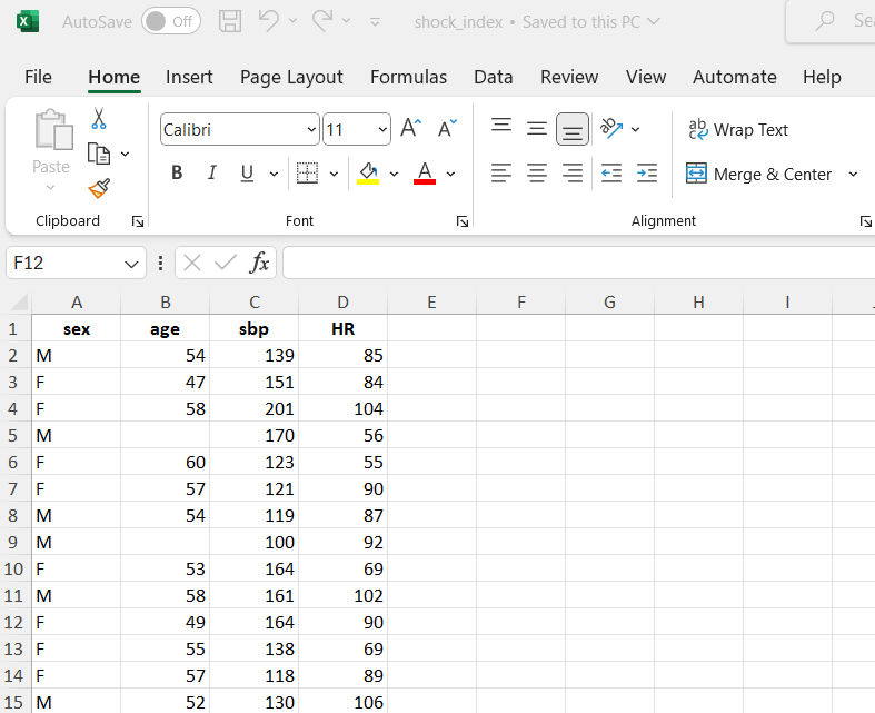
The dataset shock_index includes data regarding the characteristics of 30 adult patients with suspected pulmonary embolism. The following variables were recorded:
- sex: F for females and M for males
- age: age of the patients in years
- sbp: systolic blood pressure in mmHg
- HR: resting heart rate in beats/min
10.1.1 Importing data from Excel using the RStudio interface
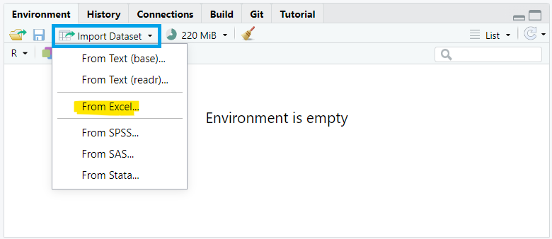
To import data using the RStudio interface, we navigate to the Environment pane, where we’ll find the “Import Dataset” button. Clicking this button will prompt a dropdown menu with options to import data from various file formats such as CSV, Excel, or other common formats. We select “From Excel…” (Figure 10.2).
A dialog box then appears, enabling us to navigate our file system and select the desired dataset. Once selected, we confirm the import by clicking “Open”. Finally, we proceed by clicking the “Import” button, which imports the selected dataset into our RStudio session.”
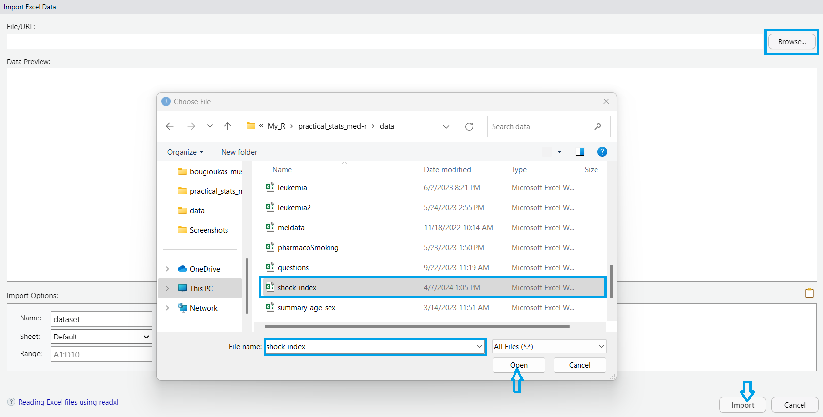
Upon successful import, the dataset will appear in the Environment pane, ready for analysis and manipulation using R’s powerful data analysis tools and functions.
10.1.2 Importing data from Excel into R with commands
Alternatively, if the dataset is saved in the subfolder named “data” of our RStudio project (see Chapter 2), we can read it with the read_excel() function from readxl package as follows:
Using head() is a convenient way to get a quick overview of our dataset and check for any obvious issues before proceeding with further analysis or data manipulation.
head(dat)# A tibble: 6 × 4
sex age sbp HR
<chr> <dbl> <dbl> <dbl>
1 M 54 139 85
2 F 47 151 84
3 F 58 201 106
4 M NA 170 56
5 F 60 123 55
6 F 57 121 90R displays the first six rows of the data frame by default. If we want to view a different number of rows (e.g., the first ten rows), we can specify the desired number as an argument as follows:
head(dat, 10)# A tibble: 10 × 4
sex age sbp HR
<chr> <dbl> <dbl> <dbl>
1 M 54 139 85
2 F 47 151 84
3 F 58 201 106
4 M NA 170 56
5 F 60 123 55
6 F 57 121 90
7 M 54 119 85
8 M NA 100 92
9 F 53 164 72
10 M 58 161 102When working with large datasets in R, it’s often useful to inspect the last few rows of a data frame. The tail() function is used for this purpose:
tail(dat)# A tibble: 6 × 4
sex age sbp HR
<chr> <dbl> <dbl> <dbl>
1 M 58 119 87
2 F 48 104 93
3 F 55 164 69
4 M 59 92 119
5 F 48 127 109
6 F 51 136 60Now, R displays the last six rows of the data frame by default.
10.2 Basic data manipulations
10.2.1 Adding an unique identifier for each observation
A unique identifier for each observation is often useful for various data manipulation and analysis tasks. In R, we can add row numbers starting from 1 to the number of rows in our data frame using the rowid_to_column() function from the tibble package:
library(tibble)
dat <- rowid_to_column(dat)
dat
# A tibble: 30 × 5
rowid sex age sbp HR
<int> <chr> <dbl> <dbl> <dbl>
1 1 M 54 139 85
2 2 F 47 151 84
3 3 F 58 201 106
4 4 M NA 170 56
5 5 F 60 123 55
6 6 F 57 121 90
7 7 M 54 119 85
8 8 M NA 100 92
9 9 F 53 164 72
10 10 M 58 161 102
# ℹ 20 more rows10.2.2 Renaming variables and cleaning names
# A tibble: 30 × 5
   patient_ID sex     age   sbp Heart.Rate
        <int> <chr> <dbl> <dbl>      <dbl>
 1          1 M        54   139         85
 2          2 F        47   151         84
 3          3 F        58   201        106
 4          4 M        NA   170         56
 5          5 F        60   123         55
 6          6 F        57   121         90
 7          7 M        54   119         85
 8          8 M        NA   100         92
 9          9 F        53   164         72
10         10 M        58   161        102
# ℹ 20 more rowslibrary(janitor)
dat <- clean_names(dat)
dat# A tibble: 30 × 5
patient_id sex age sbp heart_rate
<int> <chr> <dbl> <dbl> <dbl>
1 1 M 54 139 85
2 2 F 47 151 84
3 3 F 58 201 106
4 4 M NA 170 56
5 5 F 60 123 55
6 6 F 57 121 90
7 7 M 54 119 85
8 8 M NA 100 92
9 9 F 53 164 72
10 10 M 58 161 102
# ℹ 20 more rows10.2.3 Converting to the appropriate data type
We might have noticed that the categorical variable sex is coded as F (for females) and M (for males), so it is recognized of character type. We can use the factor() function to encode a variable as a factor:
# A tibble: 30 × 5
   patient_id sex      age   sbp heart_rate
        <int> <fct>  <dbl> <dbl>      <dbl>
 1          1 male      54   139         85
 2          2 female    47   151         84
 3          3 female    58   201        106
 4          4 male      NA   170         56
 5          5 female    60   123         55
 6          6 female    57   121         90
 7          7 male      54   119         85
 8          8 male      NA   100         92
 9          9 female    53   164         72
10         10 male      58   161        102
# ℹ 20 more rows
10.3 Basic data transformations
10.3.1 Subsetting observations (rows)
A. Select observations by indexing position within square brackets
Just as we use square brackets [row, column] to select elements from matrices, we employ the same approach to select elements from a data frame. For example, by specifying the row indices [5:10, ] within the brackets, we can efficiently access the required data for rows 5 through 10:
dat1 <- dat[5:10, ]
dat1
# A tibble: 6 × 5
patient_id sex age sbp heart_rate
<int> <fct> <dbl> <dbl> <dbl>
1 5 female 60 123 55
2 6 female 57 121 90
3 7 male 54 119 85
4 8 male NA 100 92
5 9 female 53 164 72
6 10 male 58 161 102B. Select observations by indexing with conditions within the square brackets
dat2 <- dat[which(dat$age > 55), ]
dat2
# A tibble: 11 × 5
patient_id sex age sbp heart_rate
<int> <fct> <dbl> <dbl> <dbl>
1 3 female 58 201 106
2 5 female 60 123 55
3 6 female 57 121 90
4 10 male 58 161 102
5 13 female 57 118 89
6 17 male 56 126 107
7 19 male 59 138 85
8 20 male 56 153 85
9 24 female 57 121 90
10 25 male 58 119 87
11 28 male 59 92 119dat3 <- dat[which(dat$age > 55 & dat$sex == "female"), ]
dat3# A tibble: 5 × 5
patient_id sex age sbp heart_rate
<int> <fct> <dbl> <dbl> <dbl>
1 3 female 58 201 106
2 5 female 60 123 55
3 6 female 57 121 90
4 13 female 57 118 89
5 24 female 57 121 90C. Select observations using the subset() function
dat4 <- subset(dat, age > 55)
dat4
# A tibble: 11 × 5
patient_id sex age sbp heart_rate
<int> <fct> <dbl> <dbl> <dbl>
1 3 female 58 201 106
2 5 female 60 123 55
3 6 female 57 121 90
4 10 male 58 161 102
5 13 female 57 118 89
6 17 male 56 126 107
7 19 male 59 138 85
8 20 male 56 153 85
9 24 female 57 121 90
10 25 male 58 119 87
11 28 male 59 92 119dat5 <- subset(dat, age > 55 & sex == "female")
dat5# A tibble: 5 × 5
patient_id sex age sbp heart_rate
<int> <fct> <dbl> <dbl> <dbl>
1 3 female 58 201 106
2 5 female 60 123 55
3 6 female 57 121 90
4 13 female 57 118 89
5 24 female 57 121 90D. Select observations using the filter() function from {dplyr} package
We pass the data frame first and then one or more conditions separated by a comma:
dat6 <- filter(dat, age > 55)
dat6
# A tibble: 11 × 5
patient_id sex age sbp heart_rate
<int> <fct> <dbl> <dbl> <dbl>
1 3 female 58 201 106
2 5 female 60 123 55
3 6 female 57 121 90
4 10 male 58 161 102
5 13 female 57 118 89
6 17 male 56 126 107
7 19 male 59 138 85
8 20 male 56 153 85
9 24 female 57 121 90
10 25 male 58 119 87
11 28 male 59 92 119If we want to select only female patients with age > 55:
dat7 <- filter(dat, age > 55, sex == "female")
dat7
# A tibble: 5 × 5
patient_id sex age sbp heart_rate
<int> <fct> <dbl> <dbl> <dbl>
1 3 female 58 201 106
2 5 female 60 123 55
3 6 female 57 121 90
4 13 female 57 118 89
5 24 female 57 121 9010.3.2 Reordering observations (rows)
We can also sort observations in ascending or descending order of one or more variables (columns). When multiple column names are provided, each additional column helps resolve ties in preceding columns’ values. For example, we can arrange the rows of our data based on the values of sbp (in ascending order which is the default) as follows:
# A tibble: 10 × 5
   patient_id sex      age   sbp heart_rate
        <int> <fct>  <dbl> <dbl>      <dbl>
 1         16 male      48    92        122
 2         28 male      59    92        119
 3          8 male      NA   100         92
 4         26 female    48   104         93
 5         15 female    50   109        142
 6         13 female    57   118         89
 7          7 male      54   119         85
 8         25 male      58   119         87
 9          6 female    57   121         90
10         24 female    57   121         90
We can use desc() to re-arrange in descending order. For example:
# A tibble: 10 × 5
   patient_id sex      age   sbp heart_rate
        <int> <fct>  <dbl> <dbl>      <dbl>
 1          3 female    58   201        106
 2         21 male      48   201        104
 3          4 male      NA   170         56
 4         22 female    52   170         57
 5          9 female    53   164         72
 6         11 female    49   164         90
 7         27 female    55   164         69
 8         10 male      58   161        102
 9         20 male      56   153         85
10 2 female 47 151 84# A tibble: 10 × 5
patient_id sex age sbp heart_rate
<int> <fct> <dbl> <dbl> <dbl>
1 28 male 59 92 119
2 16 male 48 92 122
3 8 male NA 100 92
4 26 female 48 104 93
5 15 female 50 109 142
6 13 female 57 118 89
7 7 male 54 119 85
8 25 male 58 119 87
9 6 female 57 121 90
10 24 female 57 121 9010.3.3 Subsetting variables (columns)
A. Select or exclude variables by indexing their name within square brackets
We can select only the sex, age, heart_rate, variables from the data frame:
# A tibble: 6 × 3
  sex      age heart_rate
  <fct>  <dbl>      <dbl>
1 male      54         85
2 female    47         84
3 female    58        106
4 male      NA         56
5 female    60         55
6 female 57 90B. Select or exclude variables by indexing position within square brackets (not recommended)
By specifying the column indices, such as c(2, 3, 5), within brackets, we can select the data in columns 2, 3, and 5 as follows:
# A tibble: 6 × 3
  sex      age heart_rate
  <fct>  <dbl>      <dbl>
1 male      54         85
2 female    47         84
3 female    58        106
4 male      NA         56
5 female    60         55
6 female 57 90C. Select variables using the subset() function
# A tibble: 6 × 3
  sex      age heart_rate
  <fct>  <dbl>      <dbl>
1 male      54         85
2 female    47         84
3 female    58        106
4 male      NA         56
5 female    60         55
6 female 57 90# A tibble: 6 × 3
sex age heart_rate
<fct> <dbl> <dbl>
1 male 54 85
2 female 47 84
3 female 58 106
4 male NA 56
5 female 60 55
6 female 57 90The select argument allows the selection by indexing the columns of interest in.
D. Select variables using the select() function from {dplyr} package
In select() function we pass the data frame first and then the variables separated by commas:
10.3.4 Creating new variables
Suppose we want to create a new variable representing the ratio of heart rate to systolic blood pressure (HR/sbp), which we will call shock index. We can achieve this by using the mutate() function as follows:
# A tibble: 30 × 6
   patient_id sex      age   sbp heart_rate shock_index
        <int> <fct>  <dbl> <dbl>      <dbl>       <dbl>
 1          1 male      54   139         85        0.61
 2          2 female    47   151         84        0.56
 3          3 female    58   201        106        0.53
 4          4 male      NA   170         56        0.33
 5          5 female    60   123         55        0.45
 6          6 female    57   121         90        0.74
 7          7 male      54   119         85        0.71
 8          8 male      NA   100         92        0.92
 9          9 female    53   164         72        0.44
10         10 male      58   161        102        0.63
# ℹ 20 more rowsNext, we want to categorize the new variable considering that normal values of this index range from 0.5 to 0.7 (beats/mmHg*min).
dat19 <- mutate(dat18,
                shock_index2 = cut(shock_index, breaks = c(-Inf, 0.5, 0.7, Inf),
                                   labels = c("low","normal","high"))
               )
dat19
# A tibble: 30 × 7
patient_id sex age sbp heart_rate shock_index shock_index2
<int> <fct> <dbl> <dbl> <dbl> <dbl> <fct>
1 1 male 54 139 85 0.61 normal
2 2 female 47 151 84 0.56 normal
3 3 female 58 201 106 0.53 normal
4 4 male NA 170 56 0.33 low
5 5 female 60 123 55 0.45 low
6 6 female 57 121 90 0.74 high
7 7 male 54 119 85 0.71 high
8 8 male NA 100 92 0.92 high
9 9 female 53 164 72 0.44 low
10 10 male 58 161 102 0.63 normal
# ℹ 20 more rows10.4 Using the native pipe operator in a sequence of commands
Given that each verb in dplyr specializes in a particular task, addressing complex queries often typically involves integrating several verbs, a process simplified by using the native pipe operator, |>. For example, we want to filter the original dataset to include only rows where the shock index category is “low” or “high”, using a sequence of dplyr verbs.
We would read this sequence as:
Begin with the dataset
datthenUse it as input to the
mutate()function to calculate theshock_indexvariable and create theshock_index2categorical variable, thenUse this output as the input to the
filter()function to select patients with “low” or “high” value of shock index.
print(sub_dat, n = Inf)# A tibble: 21 × 7
patient_id sex age sbp heart_rate shock_index shock_index2
<int> <fct> <dbl> <dbl> <dbl> <dbl> <fct>
1 4 male NA 170 56 0.33 low
2 5 female 60 123 55 0.45 low
3 6 female 57 121 90 0.74 high
4 7 male 54 119 85 0.71 high
5 8 male NA 100 92 0.92 high
6 9 female 53 164 72 0.44 low
7 13 female 57 118 89 0.75 high
8 14 male 52 130 106 0.82 high
9 15 female 50 109 142 1.3 high
10 16 male 48 92 122 1.33 high
11 17 male 56 126 107 0.85 high
12 18 female 54 139 61 0.44 low
13 22 female 52 170 57 0.34 low
14 23 male 55 122 56 0.46 low
15 24 female 57 121 90 0.74 high
16 25 male 58 119 87 0.73 high
17 26 female 48 104 93 0.89 high
18 27 female 55 164 69 0.42 low
19 28 male 59 92 119 1.29 high
20 29 female 48 127 109 0.86 high
21 30 female 51 136 60 0.44 low Alternatively we can use the %in% operator. This operator helps us to easily create multiple OR arguments:
dat |>
  mutate(shock_index = round(heart_rate / sbp, digits = 2),
         shock_index2 = cut(shock_index, breaks = c(-Inf, 0.5, 0.7, Inf),
                            labels = c("low","normal","high"))
  ) |>
  filter(shock_index2 %in% c("low", "high"))
# A tibble: 21 × 7
patient_id sex age sbp heart_rate shock_index shock_index2
<int> <fct> <dbl> <dbl> <dbl> <dbl> <fct>
1 4 male NA 170 56 0.33 low
2 5 female 60 123 55 0.45 low
3 6 female 57 121 90 0.74 high
4 7 male 54 119 85 0.71 high
5 8 male NA 100 92 0.92 high
6 9 female 53 164 72 0.44 low
7 13 female 57 118 89 0.75 high
8 14 male 52 130 106 0.82 high
9 15 female 50 109 142 1.3 high
10 16 male 48 92 122 1.33 high
# ℹ 11 more rows10.5 Reshaping data
In a pre-post test study investigating the effects of margarine consumption on blood total cholesterol (TCH) levels, eighteen participants completed a 12-week dietary intervention. Before beginning the specialized diet, baseline measurements of blood total cholesterol (in mmol/L) were recorded for each participant (week 0). Follow-up evaluations took place at the 6-week and 12-week intervals, enabling the assessment of changes in cholesterol levels during the intervention period. The collected data were organized and stored within an Excel spreadsheet, structured as follows:
dat_TCH <- read_excel(here("data", "cholesterol.xlsx"))
head(dat_TCH)
# A tibble: 6 × 3
week0 week6 week12
<dbl> <dbl> <dbl>
1 6.42 5.83 5.75
2 6.76 6.2 6.13
3 6.56 5.83 5.71
4 4.8 4.27 4.15
5 8.43 7.71 7.67
6 7.49 7.12 7.05We observe that the data set is structured in what is commonly referred to as a “wide” format. The wide format of the data is particularly suited for a repeated measures design, also known as a longitudinal or within-subject design. In such a design, the same individuals are measured multiple times over a period, with each measurement representing a different time point.
10.5.1 Ensuring that every row has a unique identifier
Before proceeding with data manipulation and analysis tasks, we create a new column in the data set that assigns a unique identifier to each row using the rowid_to_column() function:
dat_TCH <- dat_TCH |>
  rowid_to_column()
head(dat_TCH)
# A tibble: 6 × 4
rowid week0 week6 week12
<int> <dbl> <dbl> <dbl>
1 1 6.42 5.83 5.75
2 2 6.76 6.2 6.13
3 3 6.56 5.83 5.71
4 4 4.8 4.27 4.15
5 5 8.43 7.71 7.67
6 6 7.49 7.12 7.0510.5.2 From wide to long format
Wide format data may not always be the most suitable data shape for certain types of statistical analyses or visualizations compared to “long” format data. In long format, each row typically represents a single observation, while another variable denotes different time points or conditions.
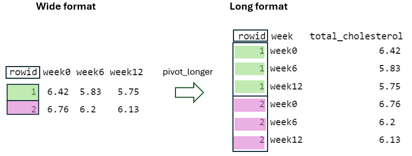
Now, let’s reshape the dataset from a wide format to a long format.
library(tidyr)
dat_TCH2_long <- dat_TCH |>
  pivot_longer(
    cols = starts_with("week"),
    names_to = "week",
    values_to = "total_cholesterol"
  )
head(dat_TCH2_long)
# A tibble: 6 × 3
rowid week total_cholesterol
<int> <chr> <dbl>
1 1 week0 6.42
2 1 week6 5.83
3 1 week12 5.75
4 2 week0 6.76
5 2 week6 6.2
6 2 week12 6.13To understand how the reshaping process works, it’s helpful to break down the pivot_longer() function with its arguments:
The argument cols = starts_with("week") specifies which columns in the original data should be pivoted. In this instance, we select the columns that start with the prefix “week”, such as “week0”, “week6”, and “week12”.
First, the values within the identifier column (rowid) of wide format need to be repeated in the long format as many times as the number of columns being pivoted, which in this case is three (Figure 10.4).
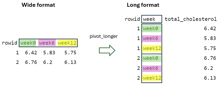
By using the argument names_to = "week", the column names being pivoted (i.e., week0, week6, and week12) become values within a newly defined variable in the long format with the name week. They are repeated as many times as the number of rows in the wide format, which in this case is two (Figure 10.5).
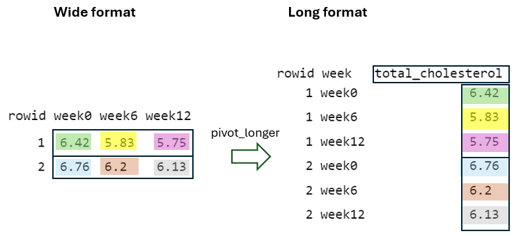
Finally, by using the argument values_to = "total_cholesterol", the cell values from the pivoted variables are placed into a newly defined variable in the long format with the name total_cholesterol (Figure 10.6).
10.5.3 From long to wide format
dat_TCH2_long |>
  pivot_wider(
    names_from = week,
    values_from = total_cholesterol
    )
# A tibble: 18 × 4
rowid week0 week6 week12
<int> <dbl> <dbl> <dbl>
1 1 6.42 5.83 5.75
2 2 6.76 6.2 6.13
3 3 6.56 5.83 5.71
4 4 4.8 4.27 4.15
5 5 8.43 7.71 7.67
6 6 7.49 7.12 7.05
7 7 8.05 7.25 7.1
8 8 5.05 4.63 4.67
9 9 5.77 5.31 5.33
10 10 3.91 3.7 3.66
11 11 6.77 6.15 5.96
12 12 6.44 5.59 5.64
13 13 6.17 5.56 5.51
14 14 7.67 7.11 6.96
15 15 7.34 6.84 6.82
16 16 6.85 6.4 6.29
17 17 5.13 4.52 4.45
18 18 5.73 5.13 5.17