# packages for graphs and tables
library(ggExtra)
library(janitor)

# packages for reliability analysis
library(irr)
library(irrCAC)
library(SimplyAgree)
library(blandr)
library(BlandAltmanLeh)
library(flextable)
library(vcd)

# packages for data import and manipulation
library(here)
library(tidyverse)35 Measures of reliability
In this chapter, we explore measures of relative and absolute reliability (or agreement) that are used to assess the consistency, stability, and reproducibility of measurements or judgments.
When we have finished this Chapter, we should be able to:
35.1 Relative and absolute reliability
Two distinct types of reliability are used: the relative and absolute reliability (agreement) (Kottner and Streiner 2011).
Relative Reliability is defined as the ratio of variability between scores of the same subjects (e.g., by different raters or at different times) to the total variability of all scores in the sample. Reliability coefficients, such as the intra-class correlation coefficient for numerical data or Cohen’s kappa for categorical data, are employed as suitable metrics for this purpose.
Absolute Reliability (or Agreement) pertains to the assessment of whether scores, or judgments are identical or comparable, as well as the extent to which they might differ. Typical statistical measures employed to quantify this degree of error are the standard error of measurement (SEM) and the limits of agreement (LOA) for numerical data.
35.2 Packages we need
We need to load the following packages:
35.3 Reliability for continuous measurements
35.3.1 Research question
The parent version of Gait Outcomes Assessment List questionnaire (GOAL) is a parent-reported outcome assessment of family priorities and functional mobility for ambulatory children with cerebral palsy. We aim to examine the test–retest reliability of the GOAL questionnaire for the total score (score range: 0 - 100) which is an indicator of the stability of the questionnaire.
Test-Retest Reliability
Test-retest reliability is used to assess the consistency and stability of a measurement tool (e.g. self-report survey instrument) over time on the same subjects under the same conditions. Specifically, assessing test-retest reliability involves administering the measurement tool to a group of individuals initially (time 1), subsequently reapplying it to the same group at a later time (time 2), and finally examining the correlation between the two sets of scores obtained.
35.3.2 Preparing the data
The GOAL questionnaire was completed twice, 30 days apart, in a prospective cohort study of 127 caregivers of children with cerebral palsy and the data were recorded as follows:
library(readxl)
goal <- read_excel(here("data", "goal.xlsx"))We will begin our investigation into the association between the first (GOAL1) and the second (GOAL2) measurement by generating a scatter plot:
ggplot(goal, aes(GOAL1, GOAL2)) +
  geom_point(color = "black", size = 2) +
  lims(x = c(0, 100), y = c(0,100)) +
  geom_abline(intercept = 0, slope = 1, linewidth = 1.0, color = "blue") +
  coord_fixed(ratio = 1)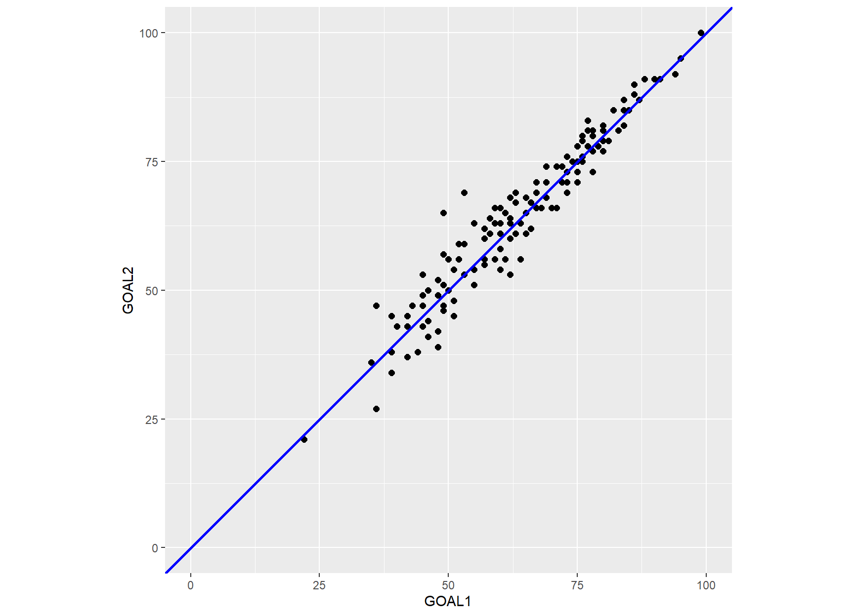
The scatter plot compares the GOAL1 and GOAL2 total scores. The solid blue diagonal line is the line of equality (i.e. the reference line: Y = X) that represents a perfect agreement of the two measurements.
35.3.3 True measurement and the measurement error
The observed scores (X) from an instrument are thought to be composed of the underlying true score (T) and the total (systematic and random) error of a measurement (E):
If the true measurement and the error term are uncorrelated, the measurement variance,
35.3.4 Intra-class correlation coefficient (ICC)
Test-retest data of continuous measurements is often assessed using the intra-class correlation coefficient
The
- one-way random effects model ICC(1)
- two-way random effects model ICC(A,1)
- two-way mixed-effects model ICC(C,1)
where A stands for “Agreement” and C stands for “Consistency”.
The choice of the appropriate ICC model depends on several factors, including how the data were collected, which variance components are considered relevant, and the specific type of reliability (agreement or consistency) we intend to assess (Liljequist, Elfving, and Skavberg Roaldsen 2019).
In the context of our example, it is recommended to use the “two-way” model rather than the “one-way” model and “agreement” rather than “consistency”, as systematic differences in the individual scores on the GOAL instrument over time are of interest (Qin et al. 2018).
For this model the Equation 35.1 becomes:
where
The variance
In population, the intra-class coefficient,
where
A statistical estimate of the
where
The Table 35.2 provides a categorization of ICC index (Koo and Li 2016), yet the interpretation of ICC values can be somewhat arbitrary.
| ICC | Level of agreement |
|---|---|
| <0.50 | Poor |
| 0.50 - 0.74 | Moderate |
| 0.75 - 0.89 | Good |
| 0.90 - 1.00 | Very good |
In R:
First, we convert data from a wide format to a long format using the pivot_longer() function:
# convert data into long format
goal_long <- goal |>
  mutate(ID = row_number()) |>
  pivot_longer(cols = c("GOAL1", "GOAL2"),
             names_to = "M", values_to = "score") |>
  mutate(ID = as.factor(ID),
         M = factor(M))

head(goal_long)
# A tibble: 6 × 3
ID M score
<fct> <fct> <dbl>
1 1 GOAL1 22
2 1 GOAL2 21
3 2 GOAL1 36
4 2 GOAL2 27
5 3 GOAL1 35
6 3 GOAL2 36Then, a two-way analysis of variance is applied with factors the id and the items:
             Df Sum Sq Mean Sq F value Pr(>F)
ID          126  58691   465.8  49.219 <2e-16 ***
M             1     34    34.1   3.598 0.0601 .
Residuals   126   1192     9.5
---
Signif. codes:  0 '***' 0.001 '**' 0.01 '*' 0.05 '.' 0.1 ' ' 1
The statistical results are arranged within a matrix and we extract the mean squares of interest:
     [,1]        [,2]      [,3]      [,4]         [,5]
[1,]  126 58691.37795 465.80459 49.219201 6.192816e-72
[2,]    1    34.05118  34.05118  3.598015 6.013766e-02
[3,]  126  1192.44882   9.46388        NA           NA
MSB <- stats[1,3]
MSM <- stats[2,3]
MSE <- stats[3,3]Finally, we calculate the ICC(A, 1) for agreement based on the Equation 35.5:
n <- dim(goal)[1]
k <- dim(goal)[2]

iccA1 <- (MSB - MSE)/(MSB + (k - 1) * MSE + k/n * (MSM - MSE))
iccA1
[1] 0.959393Next, we present R functions to carry out all the tasks for an reliability analysis.
The test–retest relative reliability obtained between the initial measurement and the measurement recorded 30 days later was very good according to the inter-rater correlation coefficient, ICC(A,1) = 0.96 (95% CI = 0.94–0.97).
35.3.5 Standard Error of Measurement (SEM)
The standard error of measurement (SEM; not to be confused with the standard error of the mean) is considered a measure that quantifies the amount of measurement error within an instrument, thus serving as an absolute estimate of the instrument’s reliability. The SEM is defined as the square root of the error variance (Lek and Van De Schoot 2018):
Now, let’s see how the SEM and
We multiply and divide the right-hand side of the equation by
and using the Equation 35.3 becomes:
Finally, the SEM is obtained by calculating the square root of both sides of the equation Equation 35.8:
If
# choose the higher standard deviation between GOAL1 and GOAL2
SD <- max(c(sd(goal$GOAL1), sd(goal$GOAL2)))

# calculate the Standard Error of Measurement for agreement
sem <- SD * sqrt(1 - iccA1)
sem
[1] 3.14089Note that the higher the ICC, the smaller the SEM which implies higher reliability as it indicates that observed scores are close to the true scores. SEM estimates the variability of the observed scores likely to be obtained given an individual’s true score (McManus 2012; Harvill 1991) . In our example, the SEM is approximately 3 units. This means that, there is a probability of 0.95 of the individual’s observed score being between -6 units and +6 units of the true score (Observed score = True score ± 2SEM), assuming normally distributed errors.
35.3.6 Minimum Detectable Change (MDC)
Now, the question that arises is whether a given change in score between test and retest is likely to be beyond the expected level of measurement error (real difference). In this case, the key measure to consider is the minimum detectable change (MDC) defined as (Goldberg and Schepens 2011):
where
# calculate the z-value for a/2 = 0.05/2 = 0.025
z <- qnorm(0.025, mean = 0, sd = 1, lower.tail = FALSE)

# calculate the minimum detectable change
mdc <- sqrt(2) * z * sem
mdc
[1] 8.705942Both random and systematic errors are taken into account in the MDC. In our example, an individual change in score smaller than 9 units can be due to measurement error and may not be a real change.
35.3.7 Limits of Agreement (LOA) and Bland-Altman Plot
- Limits of Agreement (LOA)
If the differences between the two scores (GOAL1 - GOAL2) follow a normal distribution, we expect that approximately 95% of the differences will fall within the following range (see Chapter 15):
where
# calculate the mean of the differences (MD)
MD <- mean(dif)
MD
[1] -0.7322835[1] -9.259311[1] 7.794745In our example, the mean of the differences (bias) is -0.73 (i.e. the scores at retest are on average 0.73 units higher than the scores at first test), which is a small difference. Additionally, the limits of agreement indicate that 95% of the differences lie in the range of −9 units to 8 units.
- The Bland-Altman method
The Bland-Altman method uses a scatter plot to quantify the measurement bias and a range of agreement by constructing 95% limits of agreement (LOA). The basic assumption of Bland-Altman is that the differences are normally distributed .
#calculate the mean of GOAL1 and GOAL2
mean_goal12 <- (goal$GOAL1 + goal$GOAL2)/2

# create a data frame with the means and the differences
dat_BA <- data.frame(mean_goal12, dif)

# Bland-Altman plot
BA_plot <- ggplot(dat_BA, aes(x = mean_goal12, y = dif)) +
  geom_point() +
  geom_hline(yintercept = 0, color = "black", linewidth = 0.5, linetype = "dashed") +
  geom_hline(yintercept = MD, color = "blue", linewidth = 1.0) +
  geom_hline(yintercept = lower_LOA, color = "red", linewidth = 0.5) +
  geom_hline(yintercept = upper_LOA, color = "red", linewidth = 0.5) +
  labs(title = "Bland-Altman plot of test-retest reliability",
       x = "Mean of GOAL1 and GOAL2",
       y = "GOAL1 - GOAL2") +
  annotate("text", x = 90, y = 8.6, label = "Upper LOA", color = "red", size = 4.0) +
  annotate("text", x = 90, y = -8.6, label = "Lower LOA", color = "red", size = 4.0) +
  annotate("text", x = 20, y = -1.5, label = "MD", color = "blue", size = 4.0) +
  annotate("text", x = 31.2, y = -0.2, label = "bias", color = "#EA74FC", size = 4) +
  geom_segment(x = 28, y = 0.1, xend = 28, yend = -0.85, linewidth = 0.8, colour = "#EA74FC",
               arrow = arrow(length = unit(0.07, "inches"), ends = "both"))

# add a histogram on the right-hand side of the graph
ggMarginal(BA_plot, type = "density", margins = 'y',
           yparams = list(fill = "#61D04F"))
For each pair of measurements, the difference between the two measurements is plotted on the Y axis, and the mean of the two measurements on the X axis. We can check the distribution of the differences by examining the marginal green histogram on the right-hand side of the graph. In our example, the normality assumption is met; however, if the histogram is skewed or has very long tails, the assumption of Normality might not hold.
The mean of the differences (MD), represented by the solid blue line, is an estimate of the systematic bias between the two measurements (Figure 35.3). In our case, the magnitude of bias (purple arrow) has a small value (-0.73 units). The lower and upper red horizontal lines represent the upper and lower 95% limits of agreement (LOA), respectively. Under the normality assumption of the differences (green histogram), nearly 95% of the data points are likely to be within the LOAs. In our example, most of the the points are randomly scattered around the zero dashed line within the limits of agreement (−9 to 8 units), and as expected 7 out of 127 (5.5%) data points fall out of these limits.
If we want to add confidence intervals for the MD and for the lower and upper limits of agreement (Lower LOA, Upper LOA) in Figure 35.3, we can use the bland.altman.stats() function from the {BlandAltmanLeh} package which provides these intervals:
# get the confidence intervals for the MD, Low and Upper LOA
ci_lines <- bland.altman.stats(goal$GOAL1, goal$GOAL2)$CI.lines
ci_lines
lower.limit.ci.lower lower.limit.ci.upper mean.diff.ci.lower
-10.58273587 -7.93620048 -1.49627242
mean.diff.ci.upper upper.limit.ci.lower upper.limit.ci.upper
0.03170549 6.47163356 9.11816894 # define the color of the lines of the confidence intervals
ci_colors <- c("red", "red", "blue", "blue", "red", "red")
# Bland-Altman plot
BA_plot2 <- BA_plot +
geom_hline(yintercept = ci_lines, color = ci_colors, linewidth = 0.5, linetype = "dashed")
# add a histogram on the right-hand side of the graph
ggMarginal(BA_plot2, type = "density", margins = 'y',
yparams = list(fill = "#61D04F"))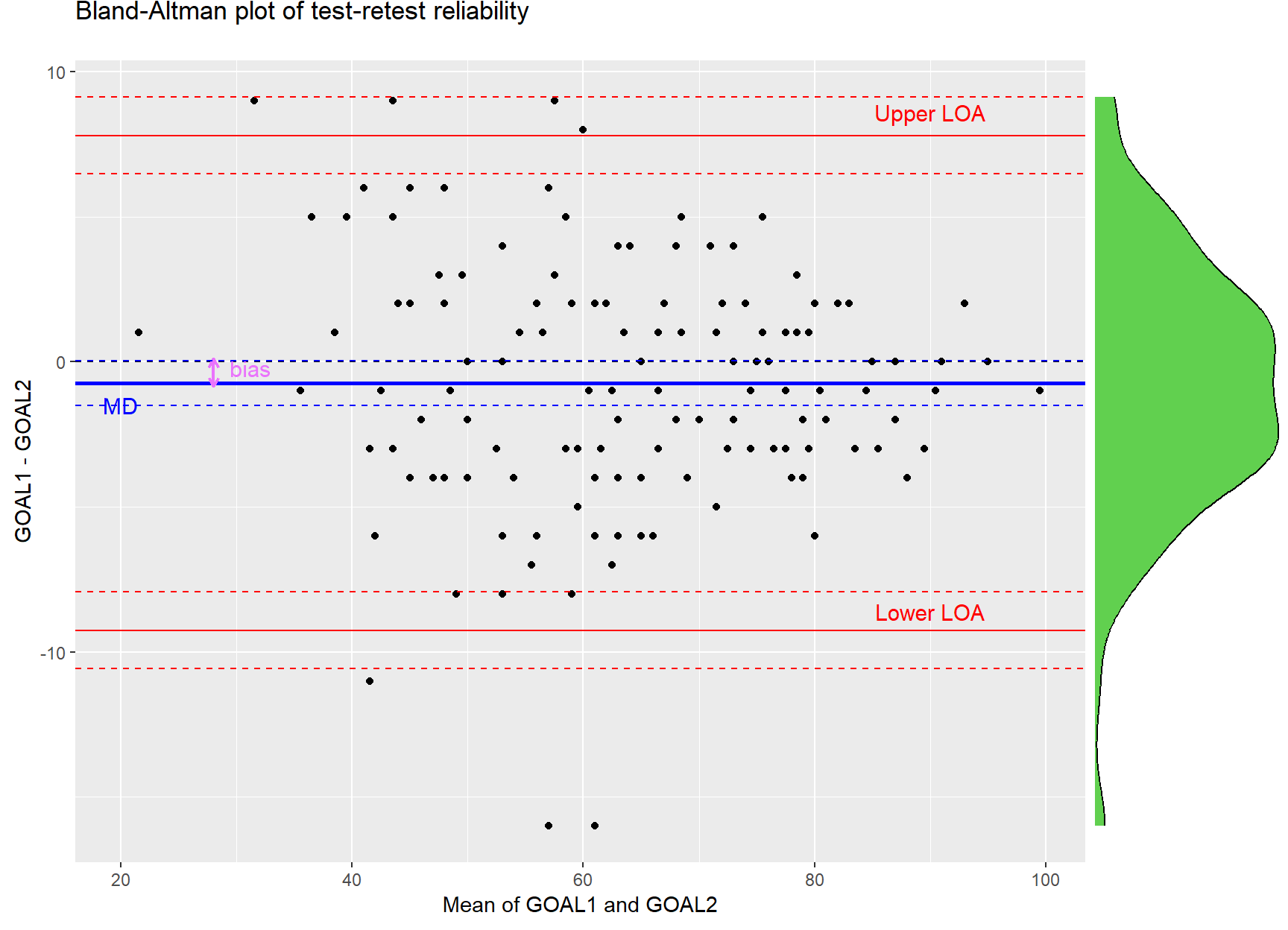
The MD (bias) can be considered insignificant, as the zero dashed line of equality lies inside the confidence interval for the mean difference (-1.5, 0.03). We can also test this with a paired t-test:
t.test(goal$GOAL1, goal$GOAL2, paired = T)
    Paired t-test

data:  goal$GOAL1 and goal$GOAL2
t = -1.8968, df = 126, p-value = 0.06014
alternative hypothesis: true mean difference is not equal to 0
95 percent confidence interval:
 -1.49627242  0.03170549
sample estimates:
mean difference
     -0.7322835
There are lots of packages on CRAN that include functions for creating Bland-Altman plots such as the blandr and {BlandAltmanLeh}:
Bland-Altman plots
blandr.draw(goal$GOAL1, goal$GOAL2) +
  annotate("text", x = 90, y = 8.6, label = "Upper LOA", color = "red", size = 4.0) +
  annotate("text", x = 90, y = -8.6, label = "Lower LOA", color = "red", size = 4.0) +
  annotate("text", x = 20, y = -1.5, label = "MD", color = "blue", size = 4.0)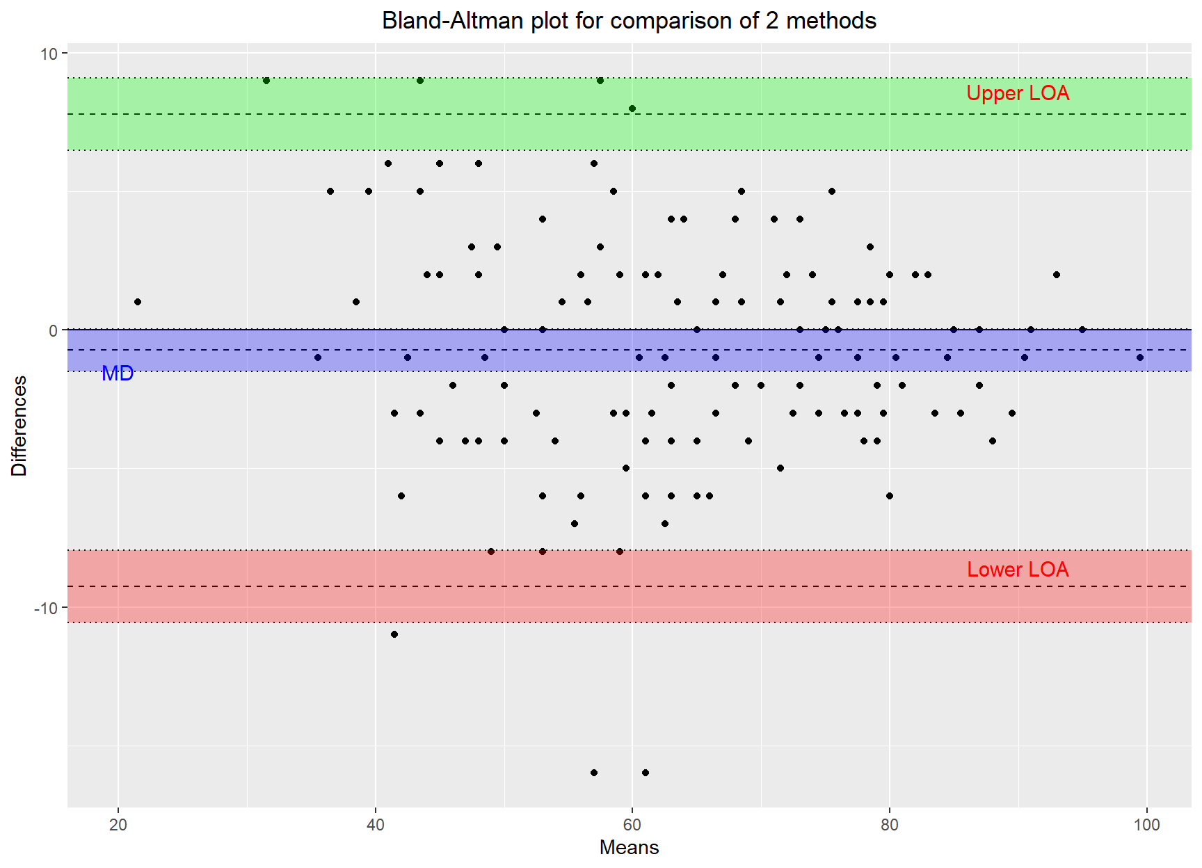
bland.altman.plot(goal$GOAL1, goal$GOAL2, graph.sys = "ggplot2", conf.int=0.95) +
  annotate("text", x = 90, y = 8.6, label = "Upper LOA", color = "red", size = 4.0) +
  annotate("text", x = 90, y = -8.6, label = "Lower LOA", color = "red", size = 4.0) +
  annotate("text", x = 20, y = -1.5, label = "MD", color = "blue", size = 4.0)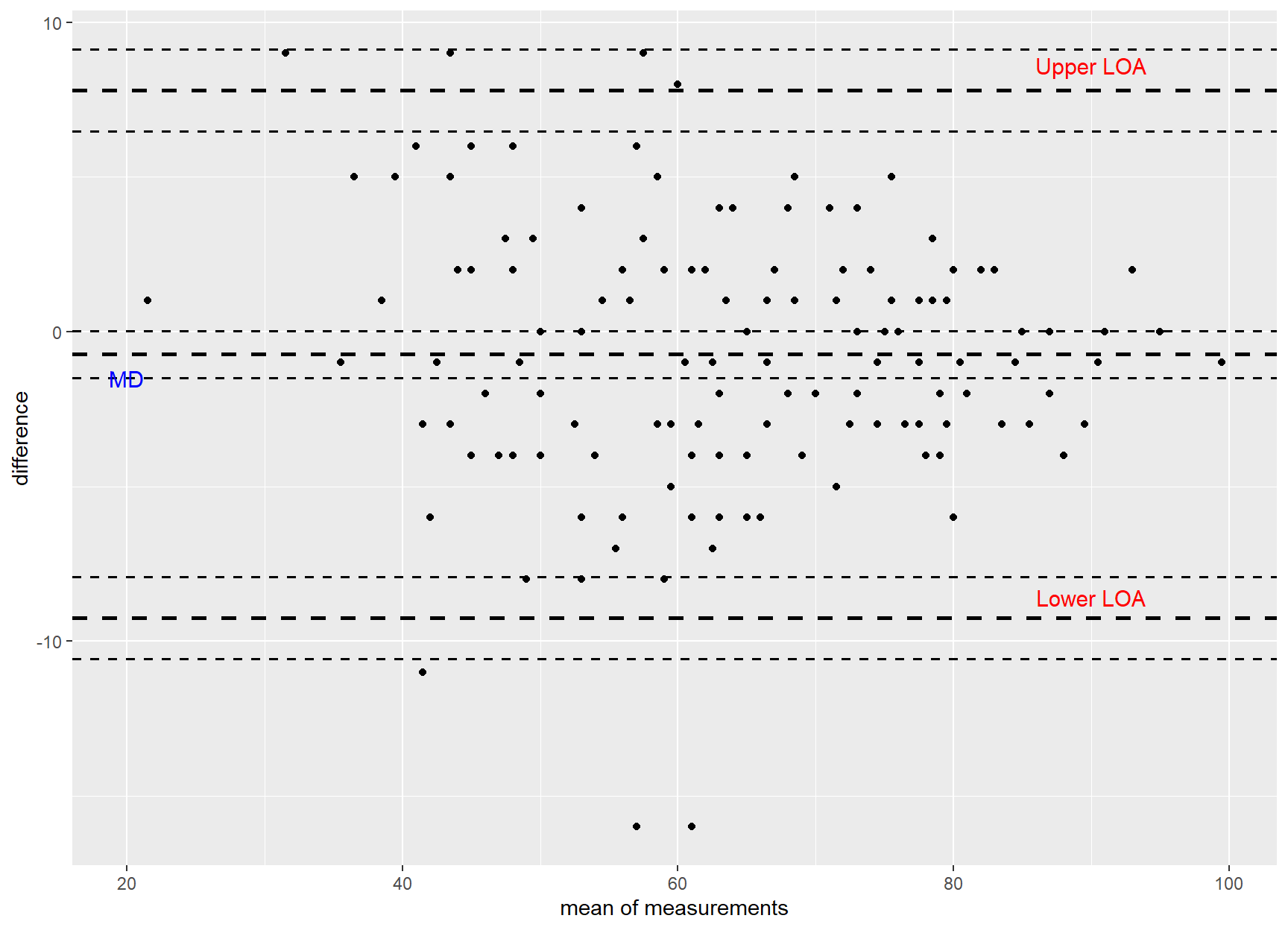
35.4 Reliability for categorical measurements
35.4.1 Research question
A screening questionnaire for Parkinson’s disease in a community was administrated with two weeks interval. We aim to examine the test–retest reliability of the following questions included in the questionnaire:
Q1: Do you have trouble buttoning buttons? (yes/no)
Q2: Do you have trouble arising from a chair? (yes/no)
Q3: Do your feet suddenly seem to freeze in door-ways? (yes/no)
Q4: Is your handwriting smaller than it once was? (yes/no)
35.4.2 Preparing the data
The file questions contains the data of the four questions which required a ‘yes’ or ‘no’ response. The same set of questions was administered to 2000 individuals aged over 65 years old on two different time points (T1 and T2) with a 14-day gap in between.
library(readxl)
qs <- read_excel(here("data", "questions.xlsx"))35.4.3 Contingency table
The test-retest data are arranged in a 2x2 contingency table as follows:
The Marginal totals (f1, f2, g1, g2) provide important summary information about the distribution of categories and rater’s assessments.
Symmetry and balance in a contingency table (Dettori and Norvell 2020)
- Symmetrical: The distribution across f1 and f2 is the same as g1 and g2
- Asymmetrical: The distribution across f1 and f2 is in the opposite direction to g1 and g2
- Balanced: The proportion of the total number of objects in f1 and g1 is equal to 0.5
- Imbalance: The proportion of the total number of objects in f1 and g1 is not equal to 0.5
35.4.4 Reliability coefficients for categorical data
Cohen’s kappa (unweighted)
The Cohen’s kappa (κ), also known as the Kappa statistic, is used to measure relative reliability for categorical items. It quantifies the degree of agreement beyond what would be expected due to chance alone (Cohen 1960).
The Cohen’s kappa statistic is defined as follows:
where
Kappa can range form negative values (no agreement) to +1 (perfect agreement).
Gwet’s AC1
Gwet’s AC1 is another measurement of relative reliability (Gwet 2008). The AC1 statistic is given by the formula:
35.4.5 Examples
Q1: Do you have trouble buttoning buttons? (symmetrical and balanced distribution of marginal totals)
The first step consists of creating the contingency table with marginal totals as follows:
qs$Q1_T1 <- factor(qs$Q1_T1, levels=c("yes", "no"))
qs$Q1_T2 <- factor(qs$Q1_T2, levels=c("yes", "no"))

table1 <- table(Q1_T1 = qs$Q1_T1, Q1_T2 = qs$Q1_T2)

tb1 <- addmargins(table1)
tb1
Q1_T2
Q1_T1 yes no Sum
yes 800 180 980
no 120 900 1020
Sum 920 1080 2000The proportions for question Q1 are:
addmargins(prop.table(table1)) Q1_T2
Q1_T1 yes no Sum
yes 0.40 0.09 0.49
no 0.06 0.45 0.51
Sum 0.46 0.54 1.00We observe that the distribution of marginal totals of question Q1 is symmetrical (f1 = 0.46 is close to g1 = 0.49; f2 = 0.54 is close to g2 = 0.51) and approximately balanced (f1 = 0.46 and f2 = 0.54 are close to 0.5; g1 = 0.49 and g2 = 0.51 are close to 0.5).
- kappa
First, we extract the elements of the tb1:
a <- tb1[1,1]
b <- tb1[1,2]
c <- tb1[2,1]
d <- tb1[2,2]
f1 <- tb1[3,1]
f2 <- tb1[3,2]
g1 <- tb1[1,3]
g2 <- tb1[2,3]
N <- tb1[3,3]
The percent of observed overall agreement is:
po <- (a + d)/N
po
[1] 0.85The proportion of agreement that would be expected by chance is:
pek <- (f1 * g1 + f2 * g2)/N^2
pek
[1] 0.5008Finally, we calculate the Cohen’s kappa statistic:
k <- (po-pek)/(1-pek)
k
[1] 0.6995192There are lots of packages on CRAN that include functions to calculate Cohen’s kappa statistic such as the irr and {vcd}:
Therefore, the relative agreement for the question Q1 is good (k = 0.7, 95%CI: 0.67, 0.73).
- AC1
For AC1 statistic, the proportion of agreement that would be expected by chance is:
q <- (f1 + g1)/(2*N)
peAC1 <- 2*q*(1-q)
peAC1
[1] 0.49875The AC1 statistic is as follows:
AC1 <- (po-peAC1)/(1-peAC1)
AC1
[1] 0.7007481We can also use the {irrCAC} package to get the relevant statistic with confidence intervals:
Q1 <- qs[1:2]
gwet.ac1.raw(Q1)$est
coeff.name pa pe coeff.val coeff.se conf.int p.value w.name
1 AC1 0.85 0.49875 0.70075 0.01596 (0.669,0.732) 0 unweightedWe conclude that AC1 is 0.7, with a 95% confidence interval ranging from 0.67 to 0.73, consistent with the result obtained using Cohen’s kappa statistic.
Q2: Do you have trouble arising from a chair? (symmetrical and imbalanced distribution of marginal totals)
qs$Q2_T1 <- factor(qs$Q2_T1, levels=c("yes", "no"))
qs$Q2_T2 <- factor(qs$Q2_T2, levels=c("yes", "no"))

table2 <- table(Q2_T1 = qs$Q2_T1, Q2_T2 = qs$Q2_T2)

tb2 <- addmargins(table2)
tb2
Q2_T2
Q2_T1 yes no Sum
yes 1600 200 1800
no 100 100 200
Sum 1700 300 2000The proportions for question Q2 are:
addmargins(prop.table(table2)) Q2_T2
Q2_T1 yes no Sum
yes 0.80 0.10 0.90
no 0.05 0.05 0.10
Sum 0.85 0.15 1.00The percent of observed overall agreement is 0.80 + 0.05 = 0.85. The distribution of marginal totals of question Q2 is symmetrical (f1 = 0.85 is close to g1 = 0.90; f2 = 0.15 is close to g2 = 0.10) but imbalanced (f1 = 0.85 and f2 = 0.15 deviate greatly from 0.5; g1 = 0.90 and g2 = 0.10 are far away from 0.5).
- kappa
Q2 <- qs[3:4]
kappa2(Q2)
Cohen's Kappa for 2 Raters (Weights: unweighted)
Subjects = 2000
Raters = 2
Kappa = 0.318
z = 14.6
p-value = 0 According to the value of kappa statistic, k = 0.32, there appears to be a fair agreement between test and re-test for question Q2.
The first kappa paradox
Although questions Q1 and Q2 have the same high percentage of agreement (
- AC1
gwet.ac1.raw(Q2)$est coeff.name pa pe coeff.val coeff.se conf.int p.value w.name
1 AC1 0.85 0.21875 0.808 0.01166 (0.785,0.831) 0 unweightedThe AC1 value is 0.81, which means that this measure is robust against what is known as the ‘kappa’ paradox.
Q3: Do your feet suddenly seem to freeze in door-ways? (symmetrical and imbalanced distribution of marginal totals)
qs$Q3_T1 <- factor(qs$Q3_T1, levels=c("yes", "no"))
qs$Q3_T2 <- factor(qs$Q3_T2, levels=c("yes", "no"))

table3 <- table(Q3_T1 = qs$Q3_T1, Q3_T2 = qs$Q3_T2)

tb3 <- addmargins(table3)
tb3
Q3_T2
Q3_T1 yes no Sum
yes 900 300 1200
no 500 300 800
Sum 1400 600 2000The proportions for question Q3 are:
addmargins(prop.table(table3)) Q3_T2
Q3_T1 yes no Sum
yes 0.45 0.15 0.60
no 0.25 0.15 0.40
Sum 0.70 0.30 1.00The percent of observed overall agreement is 0.45 + 0.15 = 0.60. The distribution of marginal totals of question Q3 is relatively symmetrical (same direction) but it is imbalanced (f1 = 0.70 and f2 = 0.30 deviate greatly from 0.5).
- kappa
Q3 <- qs[5:6]
kappa2(Q3)
Cohen's Kappa for 2 Raters (Weights: unweighted)
Subjects = 2000
Raters = 2
Kappa = 0.13
z = 5.98
p-value = 2.28e-09 According to the value of kappa statistic, k = 0.13, there appears to be a poor agreement between test and re-test for question Q3.
- AC1
gwet.ac1.raw(Q3)$est coeff.name pa pe coeff.val coeff.se conf.int p.value w.name
1 AC1 0.6 0.455 0.26606 0.02313 (0.221,0.311) 0 unweighted
Q4: Is your handwriting smaller than it once was? (asymmetrical and imbalanced distribution of marginal totals)
qs$Q4_T1 <- factor(qs$Q4_T1, levels=c("yes", "no"))
qs$Q4_T2 <- factor(qs$Q4_T2, levels=c("yes", "no"))

table4 <- table(Q4_T1 = qs$Q4_T1, Q4_T2 = qs$Q4_T2)

tb4 <- addmargins(table4)
tb4
Q4_T2
Q4_T1 yes no Sum
yes 500 700 1200
no 100 700 800
Sum 600 1400 2000The proportions for question Q4 are:
addmargins(prop.table(table4)) Q4_T2
Q4_T1 yes no Sum
yes 0.25 0.35 0.60
no 0.05 0.35 0.40
Sum 0.30 0.70 1.00The percent of observed overall agreement is 0.25 + 0.35 = 0.60. The distribution of marginal totals of question Q4 is asymmetrical (opposite direction) and imbalanced (f1 = 0.30 and f2 = 0.70 deviate greatly from 0.5).
- kappa
# Q4: Is your handwriting smaller than it once was?
Q4 <- qs[7:8]
kappa2(Q4)
Cohen's Kappa for 2 Raters (Weights: unweighted)
Subjects = 2000
Raters = 2
Kappa = 0.259
z = 13.9
p-value = 0 According to the value of kappa statistic, k = 0.26, there appears to be a fair agreement between test and re-test for question Q3.
The asymmetrical imbalance in Q4 results in a higher value of k (0.26) compared to the more symmetrical imbalance in Q3, which yielded a lower k value (0.13).
The second kappa paradox
The k values for the same percentage of agreement (
- AC1
gwet.ac1.raw(Q4)$est coeff.name pa pe coeff.val coeff.se conf.int p.value w.name
1 AC1 0.6 0.495 0.20792 0.02215 (0.164,0.251) 0 unweighted