18 Confidence intervals
Obtaining an exact point estimate of the population parameter from just one random sample is almost unattainable. However, interval estimation allows us to provide a range of values where the parameter is expected to fall with a certain level of confidence. This can be achieved by constructing confidence intervals.
18.1 Confidence interval for mean
18.1.1 The logic behind constructing a confidence interval
We will base the construction of a confidence interval on two key concepts:
The interval is around the point estimate, which represents our best estimate of the population parameter.
The standard error is utilized to quantify the extent of variability around the point estimate.
According to the Central Limit Theorem, the sampling distribution of the mean approaches a normal distribution (Chapter 17). Furthermore, the standard deviation of this sampling distribution is the standard error of the mean,

In this case, the formula for the confidence interval (CI) of mean equals:
When the sample size n is sufficiently large, the sample mean provides a good estimate of the population mean. Additionally, if the population standard deviation σ is unknown, we can estimate it by using the sample standard deviation s, and the formula becomes:
Example
The serum creatinine of a sample of 121 elderly men has a mean of 1.15 mg/dl with a standard deviation of 0.3 mg/dl. The 95% confidence interval for the mean creatinine of this population is calculated as follows:
Lower limit of 95% CI
Upper limit of 95% CI
We are 95% confident that the mean serum creatinine is between 1.1 mg/dl and 1.2 mg/dl.
In R:
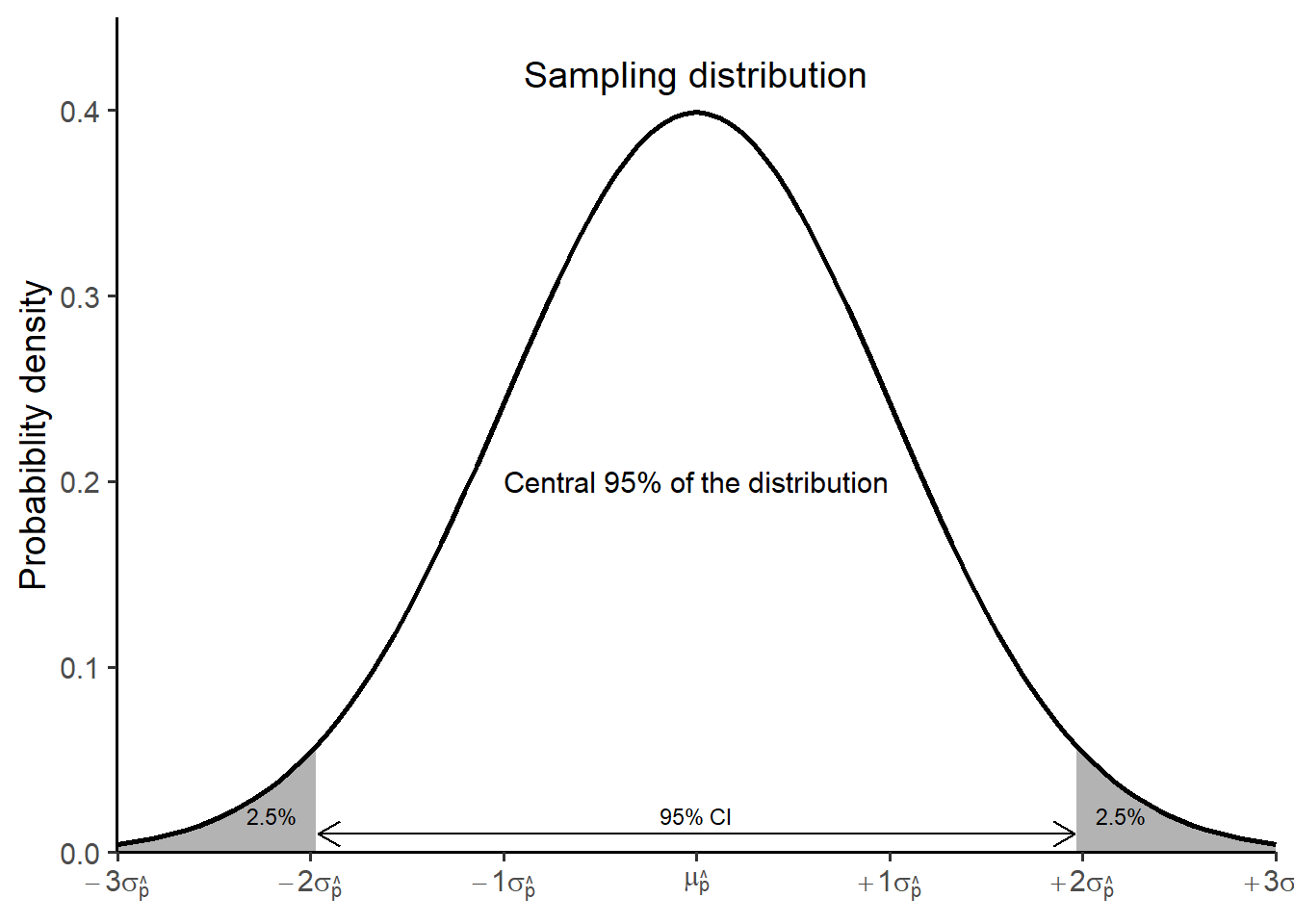
For a 95% confidence interval, each of the grey areas in Figure 18.1 equals 2.5% of the distribution because the total percentage of 5% (100-95) is equally divided between both sides of the normal distribution.
18.1.2 Confidence level
However, there is no particular reason for choosing a 95% confidence level for constructing confidence intervals other than convention; confidence levels of 90% or 99% are sometimes preferred depending on the context. For example, when a 99% confidence level is chosen, the margin of error for the mean becomes
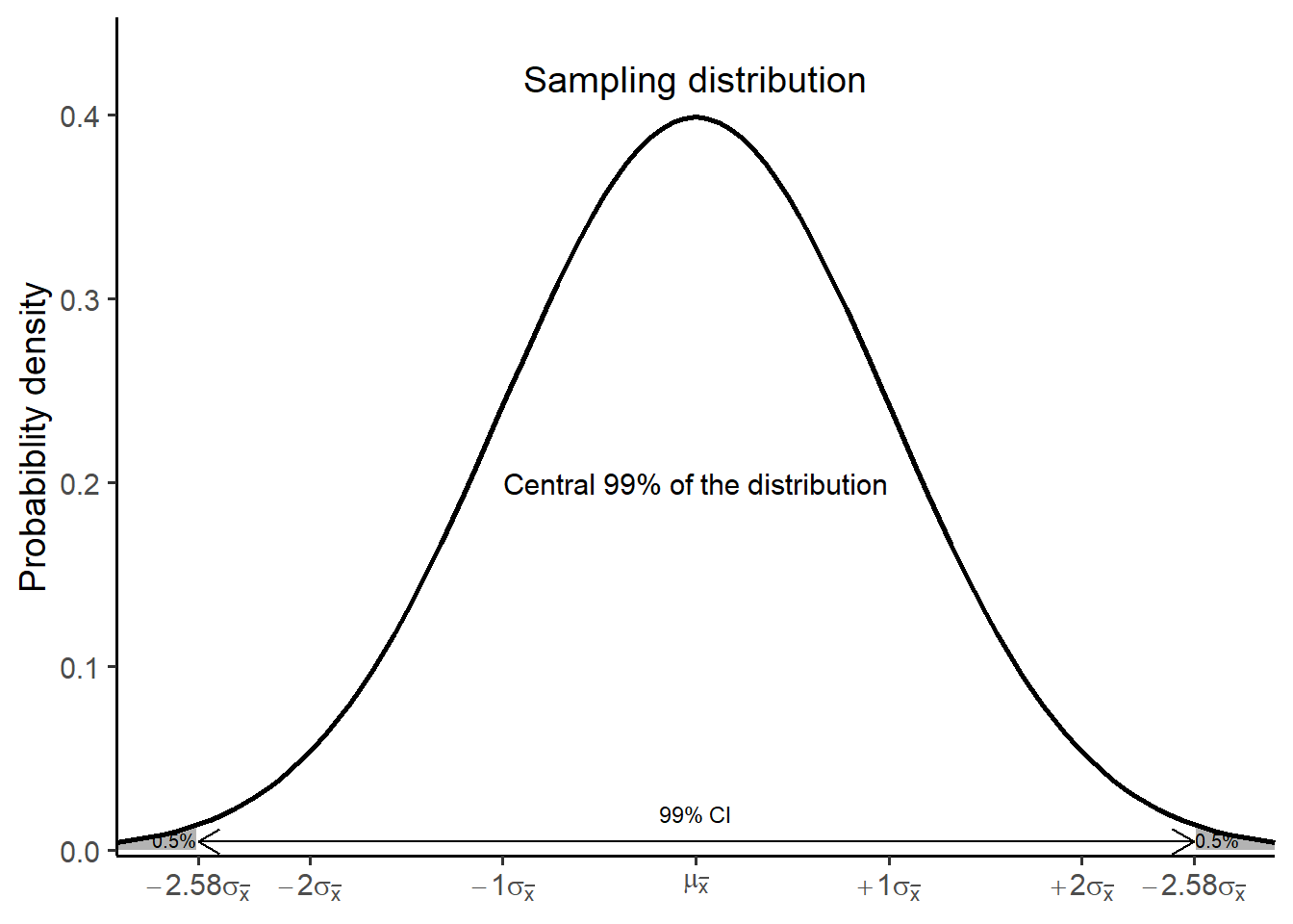
Now, each of the grey areas in Figure 18.2 equals 0.5% of the distribution because the total percentage of 1% (100-99) is equally divided between both sides of the normal distribution. In this instance, the 99% CI for the mean is:
z2 <- qnorm(0.005, lower.tail = FALSE)

# compute lower limit of 95% CI
lower_99CI <- mean - z2*(s/sqrt(n))
lower_99CI

# compute upper limit of 95% CI
upper_99CI <- mean + z2*(s/sqrt(n))
upper_99CI
[1] 1.07975
[1] 1.22025We observe that a 99% CI provides a higher level of confidence but comes with a wider range (1.07-1.22), while a 95% confidence interval offers a narrower range (1.09-1.20) but with slightly less certainty. Therefore, the increased level of confidence comes at the expense of precision, especially with smaller datasets.
18.1.3 Understanding the condidence interval
The intuitive meaning of “confidence” in a confidence interval might not be immediately clear. To understand what confidence truly represents, let’s consider once more the example of a population consisting of 100,000 adults, with a mean blood pressure (BP) of μ = 126 mmHg and a standard deviation of σ = 10 (Figure 18.3).

We proceed by generating 100 random samples of size 10 from our population distribution and construct a 95% confidence interval for the mean of each sample.
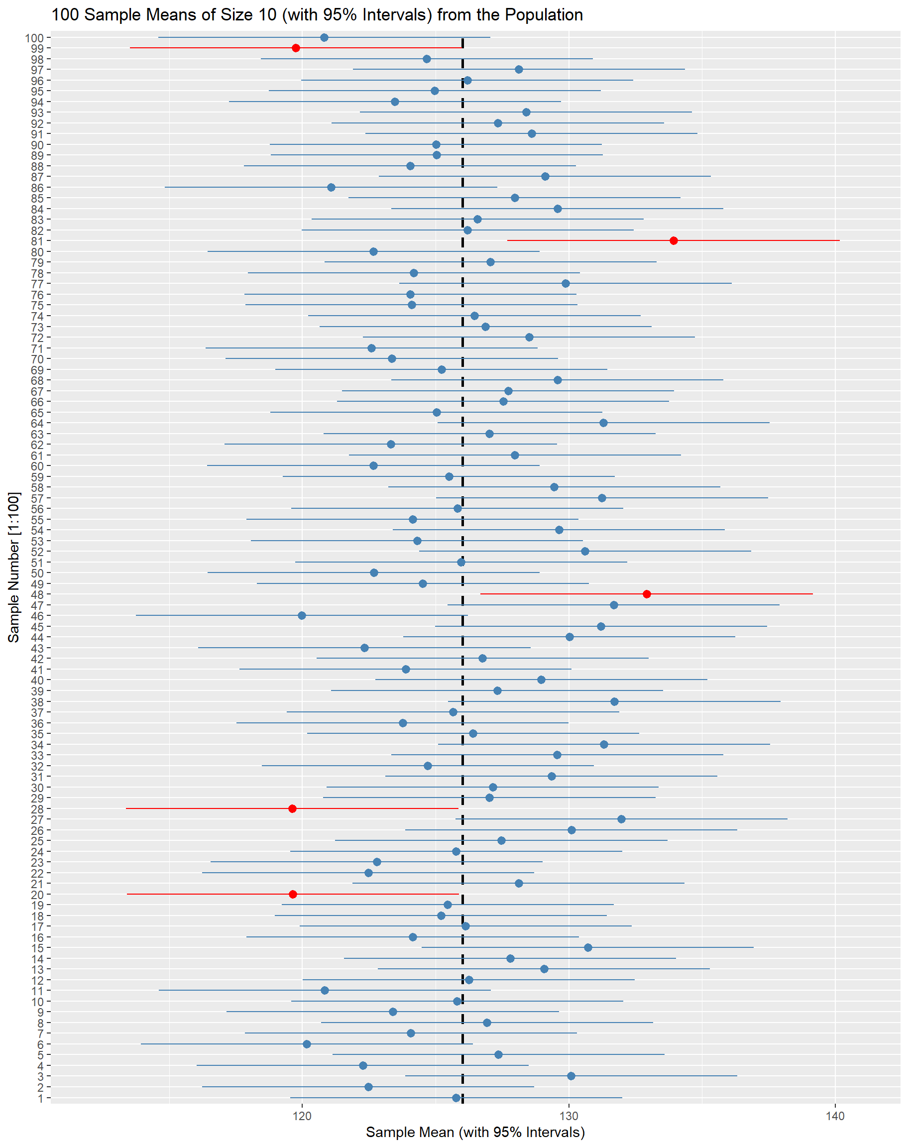
In Figure 18.4, each blue horizontal bar is a confidence interval (CI), centered on a sample mean (point). The intervals all have the same length, but are centered on different sample means as a result of random sampling from the population. The five red confidence intervals do not cover the population mean (the vertical dashed line;
18.1.4 Sample size and condidence interval
Next, we construct the 95% confidence intervals of 100 randomly generated samples of size 50 from our population (Figure 18.5):

Comparing the Figure 18.4 and Figure 18.5, we notice two key trends as the sample size increases from 10 to 50:
- The sample statistic (points) gets closer to the population parameter (black dashed line).
- The uncertainty around the estimate shrinks (confidence intervals become narrower).
A confidence interval is commonly expressed as 90% CI, 95% CI, or 99% CI, indicating the level of confidence associated with the estimate. The percentage reflects the proportion of intervals, constructed from repeated experiments, that would contain the population parameter (long-run interpretation).
Choosing an appropriate confidence level and sample size depend on the specific needs of the analysis and the trade-offs between certainty and precision.
18.2 Confidence interval for proportion (normal approximation)
Let X be a random variable representing the observed number of individuals in a sample with a binary characteristic, such as having a disease. Our best estimate of the population proportion, p, is given by the sample proportion
Similar to a confidence interval for the mean Equation 18.1, a confidence interval for a proportion can be constructed as follows:
and when the value of p is unknown, it is replaced with the sample proportion
where the standard error for proportion is
Example
Suppose a pulmonologist chooses a random sample of 317 patients from the patient register, and finds that 34 of them have a history of suffering from chronic obstructive pulmonary disease (COPD). The 95% confidence interval for the proportion of COPD is calculated as follows:
Additionally, the condition
np = 317 * 0.107 = 33.9 > 5
n(1-p) = 317 * (1 - 0.107) = 317 * 0.893 = 283 > 5
Lower limit of 95% CI
Upper limit of 95% CI
Based on our random sample, we are 95% confident that the percentage of patients with COPD falls within the range of 7.3% to 14.1%.
In R: