37 Receiver Operating Characteristic (ROC) curve
When a diagnostic test result is measured in a continuous scale, sensitivity and specificity vary with different cut-off points (thresholds). Therefore, a convenient cut-off point1 must be selected in order to calculate the measures of diagnostic accuracy of the test. Receiver operating characteristic (ROC) curve analysis can be used to help with this decision.
1 NOTE: there is critique, however, that the binary diagnosis is problematic.
When we have finished this Chapter, we should be able to:
37.1 Research question
We want to compare two screening questionnaires for chronic obstructive pulmonary disease (COPD) among smokers aged >45 years in the primary care setting:
- International Primary Care Airways Group (IPAG) questionnaire (Score: 0-38)
- COPD Population Screener (COPDPS) questionnaire (Score: 0-10)
Each participant received both questionnaires (‘fully paired’ design). The diagnosis of COPD was based on spirometric criterion (FEV 1 /FVC <0.7 following bronchodilation), clinical status (medical history, symptoms and physical examination), and exclusion of other diseases.
37.2 Packages we need
We need to load the following packages:
Other relative packages: OptimalCutpoints, cutpointr
37.3 Preparing the data
We import the data copd in R:
library(readxl)
dat <- read_excel(here("data", "copd.xlsx"))We inspect the data and the type of variables:
glimpse(dat)Rows: 2,587
Columns: 3
$ IPAG <dbl> 11, 15, 4, 7, 13, 15, 13, 14, 4, 21, 17, 11, 10, 17, 9, 18, …
$ COPDPS <dbl> 4, 3, 2, 2, 4, 4, 2, 2, 2, 6, 5, 2, 2, 4, 2, 4, 2, 5, 2, 3, …
$ diagnosis <dbl> 0, 0, 0, 0, 0, 0, 0, 0, 0, 1, 0, 0, 0, 0, 0, 0, 0, 0, 0, 0, …37.4 Using cut-off points and the ROC curve
Based on previous studies, the cut-off points for a positive response are:
- ≥ 17 for the IPAG questionnaire
- ≥ 5 for the COPDPS questionnaire.
We can evaluate these cut-off values by calculating their associated measures of diagnostic accuracy (i.e Se, Sp, PPV, NPV).
dat <- dat |>
  mutate(IPAG_cat = cut(IPAG, c(0, 17, 38), labels=c("-","+"),
                        include.lowest = TRUE, right=FALSE),
         COPDPS_cat = cut(COPDPS, c(0, 5, 10), labels=c("-","+"),
                          include.lowest = TRUE, right=FALSE))

dat <- as.data.frame(dat)

# we need to create a roc object for each questionnaire
roc1 <- roc(dat$diagnosis, dat$IPAG)
roc2 <- roc(dat$diagnosis, dat$COPDPS)For screening purposes such as mammogram, the cut-off point can be selected to favor a higher sensitivity. Thus, a negative test result indicates the absent of the disease (Se-N-out; sensitive, negative, “rule out” the disease).
For confirmative diagnosis purposes, for example, when a chemotherapy is to initiated once the diagnosis is established, the cut-off point can be selected to favor a higher specificity. Thus, a positive test result indicates the presence of disease (Sp-P-in; specificity, positive, “rule in” the disease).
Additionally, for a given diagnostic test, we can consider all cut-off points that give a unique pair of values for sensitivity and specificity. We can plot in a graph, which is known as a ROC curve, the sensitivity on the y-axis and 1-specificity (false positives) values on the x-axis for all these possible cut-off points of the diagnostic test. Then, the area under the ROC curve (AUC of ROC), also called the c-statistic, can be calculated which is widely used as a measure of overall performance.
37.4.1 IPAG questionnaire
A. The use of a cut-off value: IPAG score ≥17
First, we will find the counts of individuals in each of the four possible outcomes in a 2×2 table for the cut-off point of 17:
table(dat$IPAG_cat, dat$diagnosis)
       0    1
  - 1670   70
  +  644  203
Next, we reformat the table as follows:
tb1 <- as.table(
  rbind(c(203, 644), c(70, 1670))
  )

dimnames(tb1) <- list(
  Test = c("+", "_"),
  Outcome = c("+", "-")
)

tb1
Outcome
Test + -
+ 203 644
_ 70 1670epi.tests(tb1, digits = 3) Outcome + Outcome - Total
Test + 203 644 847
Test - 70 1670 1740
Total 273 2314 2587
Point estimates and 95% CIs:
--------------------------------------------------------------
Apparent prevalence * 0.327 (0.309, 0.346)
True prevalence * 0.106 (0.094, 0.118)
Sensitivity * 0.744 (0.687, 0.794)
Specificity * 0.722 (0.703, 0.740)
Positive predictive value * 0.240 (0.211, 0.270)
Negative predictive value * 0.960 (0.949, 0.969)
Positive likelihood ratio 2.672 (2.428, 2.940)
Negative likelihood ratio 0.355 (0.290, 0.436)
False T+ proportion for true D- * 0.278 (0.260, 0.297)
False T- proportion for true D+ * 0.256 (0.206, 0.313)
False T+ proportion for T+ * 0.760 (0.730, 0.789)
False T- proportion for T- * 0.040 (0.031, 0.051)
Correctly classified proportion * 0.724 (0.706, 0.741)
--------------------------------------------------------------
* Exact CIsThe results using the cut-off point of 17 give Se = 0.744 (0.687 - 0.794) and Sp = 0.722 (0.703 - 0.740). We observe that the probability of the absence of COPD given a negative test result is high NPV = 0.960 (95% CI: 0.949, 0.969) in this sample with smokers.
B. The area under the ROC curve of IPAG questionnaire
Let’s calculate the AUC of ROC for the IPAG questionnaire:
auc(roc1)Area under the curve: 0.7986The 95% confidence interval of this area is:
ci.auc(roc1)95% CI: 0.7687-0.8286 (DeLong)The ability of the IPAG questionnaire to discriminate between individuals with and without COPD is shown graphically by the ROC curve in (Figure 37.2):
# create the plot
g1 <- ggplot(dat, aes(d = diagnosis, m = IPAG)) +
  geom_roc(n.cuts = 0, color = "#0071BF") +
  theme(text = element_text(size = 14)) +
  geom_abline(intercept = 0, slope = 1, linetype = 'dashed') +
  scale_x_continuous(expand = c(0, 0.015)) +
  scale_y_continuous(expand = c(0, 0)) +
  labs(x = "1 - Specificity", y = "Sensitivity")

# add annotations to the plot
g1 + annotate("text", x=0.70, y=0.30,
           label=paste("AUC IPAG = ", 0.799,
                       "(95% CI = ", 0.769, " - ", 0.829, ")"))
The AUC of IPAG questionnaire equals to 0.799 (95% CI: 0.769 - 0.829) which indicates a reasonable2 diagnostic test.
2 The dashed diagonal line connecting (0,0) to (1,1) in the ROC plot corresponds to a test that is completely useless in diagnosis of a disease, AUC = 0.5 (i.e. individuals with and without the disease have equal “chances” of testing positive). A test which is perfect at discriminating between those with disease and those without disease has an AUC = 1 (i.e. the ROC curve approaches the upper left-hand corner).
Youden index (J statistic), which is defined as the sum of sensitivity and specificity minus 1, is often used in conjunction with the ROC curve. The maximum value of the Youden index may be used as a criterion for selecting the optimal cut-off point (threshold) for a diagnostic test as follows:
  threshold sensitivity specificity
1      18.5   0.6739927   0.8063959
We observe that the optimal cut-off point (threshold) for this sample equals to 18.5 which is slightly higher than the value of 17 that was obtained from other studies.
We can also easily calculate the maximum value of Youden index according to the previous definition of the Youden index:
0.674 + 0.806 - 1[1] 0.48
37.4.2 COPDPS questionnaire
A. The use of a cut-off value: COPDPS score ≥5
First, we will find the counts of individuals in each of the four possible outcomes in a 2×2 table for the cut-off point of 5:
table(dat$COPDPS_cat, dat$diagnosis)
       0    1
  - 2089  121
  +  225  152
Next, we reformat the table as follows:
tb2 <- as.table(
  rbind(c(152, 225), c(121, 2089))
  )

dimnames(tb2) <- list(
  Test = c("+", "_"),
  Outcome = c("+", "-")
)

tb2
Outcome
Test + -
+ 152 225
_ 121 2089epi.tests(tb2, digits = 3) Outcome + Outcome - Total
Test + 152 225 377
Test - 121 2089 2210
Total 273 2314 2587
Point estimates and 95% CIs:
--------------------------------------------------------------
Apparent prevalence * 0.146 (0.132, 0.160)
True prevalence * 0.106 (0.094, 0.118)
Sensitivity * 0.557 (0.496, 0.617)
Specificity * 0.903 (0.890, 0.915)
Positive predictive value * 0.403 (0.353, 0.455)
Negative predictive value * 0.945 (0.935, 0.954)
Positive likelihood ratio 5.726 (4.864, 6.741)
Negative likelihood ratio 0.491 (0.430, 0.561)
False T+ proportion for true D- * 0.097 (0.085, 0.110)
False T- proportion for true D+ * 0.443 (0.383, 0.504)
False T+ proportion for T+ * 0.597 (0.545, 0.647)
False T- proportion for T- * 0.055 (0.046, 0.065)
Correctly classified proportion * 0.866 (0.853, 0.879)
--------------------------------------------------------------
* Exact CIsThe results using the cut-off point of 5 give Se = 0.577 (0.496 - 0.617) and Sp = 0.903 (0.890 - 0.915).
B. The area under the ROC curve of COPDPS questionnaire
The AUC of ROC curve of COPDPS questionnaire is:
auc(roc2)Area under the curve: 0.7908The 95% confidence interval of this area is:
ci.auc(roc2)95% CI: 0.7602-0.8214 (DeLong)The ROC curve of COPDPS questionnaire (Figure 37.3) follows:
# create the plot
g2 <- ggplot(dat, aes(d = diagnosis, m = COPDPS)) +
  geom_roc(n.cuts = 0, color = "#EFC000") +
  theme(text = element_text(size = 14)) +
  geom_abline(intercept = 0, slope = 1, linetype = 'dashed') +
  scale_x_continuous(expand = c(0, 0.015)) +
  scale_y_continuous(expand = c(0, 0)) +
  labs(x = "1 - Specificity", y = "Sensitivity")

# add annotations to the plot
g2 + annotate("text", x=0.70, y=0.25,
           label= paste("AUC COPDPS = ", 0.791,
                        "(95% CI = ", 0.760, " - ", 0.821, ")"))
The AUC of COPDPS questionnaire equals to 0.791 (95% CI: 0.760 - 0.821) which is close to the value 0.799 of AUC of IPAG questionnaire.
The optimal cut-off point using the Youden Index as best method is:
  threshold sensitivity specificity
1       4.5   0.5567766   0.9027658
We observe that the optimal cut-off point (threshold) for this sample equals to 4.5 which is close to the value of 5 that was obtained from other studies.
We can also calculate the maximum value of the Youden index:
0.557 + 0.903 - 1[1] 0.4637.5 Comparing ROC Curves
A. Graphical comparison of ROC curves
We can plot the ROC curves for both questionnaires in the same graph and compare the area under the curves (Figure 37.4):
# prepare the data
longdata <- melt_roc(dat, "diagnosis", c("IPAG", "COPDPS"))

# create the plot
g <- ggplot(longdata, aes(d = D, m = M, color = name)) +
  geom_roc(n.cuts = 0) +
  theme(text = element_text(size = 14),
        legend.position="top") +
  geom_abline(intercept = 0, slope = 1, linetype = 'dashed') +
  scale_x_continuous(expand = c(0, 0.015)) +
  scale_y_continuous(expand = c(0, 0)) +
  scale_color_jco() +
  labs(x = "1 - Specificity", y = "Sensitivity", colour="Questionnaire")

# add annotations to the plot
g + annotate("text", x=0.70, y=0.35, color = "#0071BF",
           label=paste("AUC IPAG = ", 0.799,
                       " (95% CI = ", 0.769, " - ", 0.829, ")")) +
  annotate("text", x=0.70, y=0.28, color = "#EFC000",
           label= paste("AUC COPDPS = ", 0.791,
                        "(95% CI = ", 0.760, " - ", 0.821, ")"))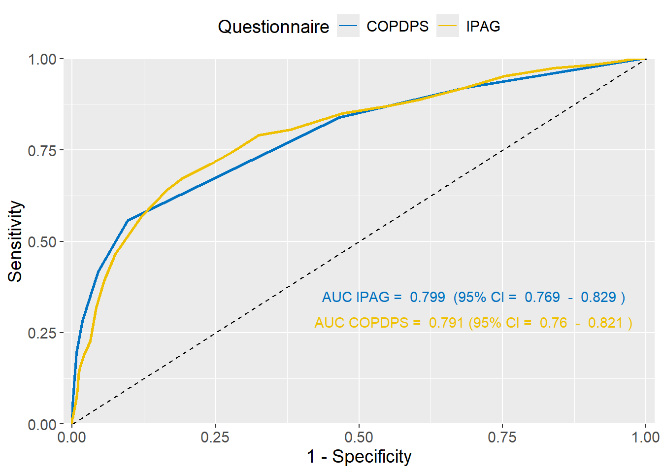
The AUC values obtained from the ROC curve were 0.799 (95% CI: 0.769 - 0.829) for the IPAG questionnaire and 0.791 (95% CI: 0.760 - 0.821) for the COPDPS questionnaire. Therefore, the two questionnaires have similar overall performance in the present sample.
B. Compare AUCs using the DeLong’ s test
The DeLong’s test can be used for comparing 2 areas under the curve (AUCs).
    DeLong's test for two correlated ROC curves

data:  roc1 and roc2
Z = 0.67525, p-value = 0.4995
alternative hypothesis: true difference in AUC is not equal to 0
95 percent confidence interval:
 -0.01488242  0.03052696
sample estimates:
AUC of roc1 AUC of roc2
  0.7986393   0.7908170
There was no significant difference in the AUC values with the two questionnaires (p = 0.45 < 0.05).