14  Probability Distributions

When we have finished this Chapter, we should be able to:

Learning objectives

• Understand and use the terminology of probability

14.1 Packages we need

We need to load the following packages:

# graphs
library(tidyverse)
library(igraph)

14.2 Random variables and Probability Distributions

A random variable assigns a numerical quantity to every possible outcome of a random phenomenon and may be:

• discrete if it takes either a finite number or an infinite sequence of possible values
• continuous if it takes any value in some interval on the real numbers

For example, a random variable representing the ABO blood system (A, B, AB, or O blood type) would be discrete, while a random variable representing the height of a person in centimeters would be continuous.

  Example

Suppose the X random variable for blood type is explicitly defined as follows:

\[X={\begin{cases}1, &for\ blood\ type\ A\\2, &for\ blood\ type\ B\\3, &for\ blood\ type\ AB\\4, &for\ blood\ type\ O\end{cases}}\]

That is, X is the discrete random variable that has four possible outcomes; it takes the value 1 if the person has blood type A, 2 if the person has blood type B, 3 if the person has blood type AB, and 4 if the person has blood type O.

We can also find the probability distribution that describes the probability of different possible values of random variable X. Note that the probability axioms and properties that we discussed earlier are also applied to random variables (e.g., the total probability for all possible values of a random variable equals to one).

Probability distributions are often presented using probability tables or graphs. For example, assume that the individual probabilities for different blood types in a population are P(A) = 0.41, P(B) = 0.10, P(AB) = 0.04, and P(O) = 0.45 (Note that: P(A) + P(B) + P(AB) + P(O) = 0.41 + 0.10 + 0.04 + 0.45 = 1).

\[P(X=x)={\begin{cases}0.41,&for\ x=1\\0.10,&for\ x=2\\0.04,&for\ x=3\\0.45,&for\ x=4\end{cases}}\]

Blood type	A	B	AB	O
X	1	2	3	4
P(X)	0.41	0.10	0.04	0.45

Here, x denotes a specific value (i.e. 1, 2, 3, or 4) of the random variable X. Then, instead of saying P(A) = 0.41, i.e., the blood type is A with probability 0.41, we can say that P(X = 1) = 0.41, i.e., X is equal to 1 with probability of 0.41.

We can use the probability distribution to answer probability questions. For example, what is the probability that a randomly selected person from the population can donate blood to someone with type B blood?

We know that individuals with blood type B or O can donate to a person with blood type B (Figure 14.1).

# data in a form of a matrix
x <- c(1, 0, 0, 0, 1, 1, 0, 0, 1, 0, 1, 0, 1, 1, 1, 1)
nodes_names <- c("O", "A", "B", "AB")
adjm <- matrix(x, 4, dimnames = list(nodes_names, nodes_names))

set.seed(124)
# build the graph object
network <- graph_from_adjacency_matrix(adjm)

# plot it
plot(network, vertex.size= 32, vertex.color = "red")

Figure 14.1: Blood types matching for a safe transfusion.

Therefore, we need to find the probability P(blood type B OR blood type O). Since the events blood type B or blood type O are mutually exclusive, we can use the addition rule for mutually exclusive events to get:

\[ \textrm{P(blood type B OR blood type O)= P(X = 2) + P(X = 4) = 0.10 + 0.45 = 0.55}\]

Hence, there is a 55% chance that a randomly selected person in our population can donate blood to someone with type B blood.

There are several types of probability distributions, and they can be broadly categorized into two main groups: discrete probability distributions and continuous probability distributions.

INFO

Degrees of freedom (i.e., the number of parameters that are free to vary) are intrinsic to probability distributions, influencing their shapes, properties, and applications in statistical analysis. For instance, in the chi-square, t, and F distributions, degrees of freedom determine their characteristics.

14.3 Discrete Probability Distributions

The probability distribution of a discrete random variable X is defined by the probability mass function (pmf) as:

\[ P(X = x) = P(x) \tag{14.1}\]

where:

\(P(X = x)\) is the probability that the random variable X takes the value x and

\(P(x)\) is the probability of the specific outcome x occurring.

The pmf has two properties:

• \(P(x) \geq 0\)
• \(\sum_{x} P(x) = 1\)

 

Additionally, the cumulative distribution function (cdf) gives the probability that the random variable X is less than or equal to x and is usually denoted as F(x):

\[F(x) = P(X \le x)= \sum_{x_i\le x} P(x_i) \tag{14.2}\]

where the sum takes place for all the values \(x_1, x_2, \ldots, x_i\), which are \(x_i\le x\).

 

When dealing with a random variable, it is common to calculate three important summary statistics: the expected value, variance and standard deviation.

Expected Value

The expected value or mean, denoted as E(X) or μ, is defined as the weighted average of the values that X can take on, with each possible value being weighted by its respective probability, P(x).

\(\mu = E(X)= \sum\limits_i x_i \cdot P(x_i)\)

Variance

We can also define the variance, denoted as \(\sigma^2\), which is a measure of the variability of the X.

\(\sigma^2=\text{Var}(X)= E[X - E(X)]^2 = E[(X - \mu)^2] = \sum\limits_i\ (x_i-\mu)^2 P(x_i)\)

There is an easier form of this formula.

\(\sigma^2=\text{Var}(X)= E(X^2) - E(X)^2=\sum\limits_i x_i^2 P(x_i)-\mu^2\)

Standard deviation

The standard deviation is the square root of the variance.

\(\sigma=\sqrt{\text{Var(X)}}=\sqrt{\sigma^2}\)

14.3.1 Bernoulli distribution

A random experiment with two possible outcomes, generally referred to as success (x = 1) and failure (x = 0), is called a Bernoulli trial.

Let X be a binary random variable of a Bernoulli trial which takes the value 1 (success) with probability p and 0 (failure) with probability 1-p. The distribution of the X variable is called Bernoulli distribution with parameter p, denoted as \(X ∼ Bernoulli(p)\), where \({0\leq p\leq 1}\).

• The probability mass function (pmf) of X is given by:

\[P(X=x)={\begin{cases}1-p,&for\ x=0\\p,&for\ x=1\end{cases}} \tag{14.3}\]

which can also be written as: \[P(X=x)=p^{x}(1-p)^{1-x}\quad {\text{for }}x\in \{0,1\} \tag{14.4}\]

 

• The cumulative distribution function (cdf) of X is given by:

\[F(x) = P(X \le x)= {\begin{cases}0,&for\ x <0\\1-p,&for\ 0\leq x < 1\\1,&for\ x \geq 1 \end{cases}} \tag{14.5}\]

Note

The random variable X can take either value 0 or value 1. If \(x<0\), then \(P(X \le x) = 0\) because X can not take values smaller than 0. If \(0\leq x < 1\), then \(P(X \le x) = P(X=0) = 1-p\). Finally, if \(x \geq 1\), then \(P(X \le x) = P(X = 0) + P(X = 1) = (1 - p) + p = 1\).

 

The expected value of random variable, X, with Bernoulli(p) distribution is:

NOTE: In this case, the mean can be interpreted as the proportion of the population who has the outcome (success).

\[μ = E(X)= p \tag{14.6}\]

Proof:

\(E(X) = \sum_{i=1}^{2}x_iP(x_i) = 0 \cdot P(X=0) + 1 \cdot P(X=1) = p\)

The variance is:

\[\sigma^2 = Var(X) = p(1-p) \tag{14.7}\]

Proof:

\(Var(X) = \sum_{i=1}^{2}x_iP(x_i) - \mu^2= 0 \cdot P(X=0) + 1 \cdot P(X=1) - p^2= p (1-p)\)

and the standard deviation is:

\[ σ = \sqrt{Var(X)} = \sqrt{p(1-p)} \tag{14.8}\]

 

  Example

Let X be a random variable representing the result of a surgical procedure, where X = 1 if the surgery was successful and X = 0 if it was unsuccessful. Suppose that the probability of success is 0.7; then X follows a Bernoulli distribution with parameter p = 0.7: \(X ∼ Bernoulli(0.7)\).

Find the main characteristics of this distribution.

• The pmf for this distribution is:

\[P(X=x)={\begin{cases}0.3,&for\ x=0\\0.7,&for\ x=1\end{cases}} \tag{14.9}\]

According to Equation 14.9 we have:

X	0	1
P(X)	0.3	0.7

 

We can plot the pmf for visualizing the distribution of the two outcomes (Figure 14.2).

# Create a data frame
x <- as.factor(c(0, 1))
y <- c(0.3, 0.7)
dat1 <- data.frame(x, y)
 
# Plot
ggplot(dat1, aes(x = x, y = y)) +
  geom_segment(aes(x = x, xend=x, y=0, yend = y), color = "black") +
  geom_point(color="deeppink", size = 4) +
  theme_classic(base_size = 14) +
  labs(title = "pmf Bernoulli(0.7)",
       x = "X", y = "Probability") +
  theme(axis.text = element_text(size = 14))

Figure 14.2: Plot of the pmf for Bernoulli(0.7) distribution.

• The cdf for this distribution is:

\[F(x) = P(X \le x)={\begin{cases}0,&for\ x <0\\0.3,&for\ 0\leq x < 1\\1,&for\ x \geq 1 \end{cases}}\]

# Create a data frame
dat2 <- data.frame(x = -1:2, 
                   y =  pbinom(-1:2, size = 1, prob = 0.7))
# Step line plot
ggplot(dat2, aes(x=x, y=y)) +
  geom_step() +
  scale_y_continuous(limits = c(0, 1), breaks = seq(0, 1, 0.1)) +
theme_classic(base_size = 14) +
  labs(title = "cdf Bernoulli(0.7)", 
       x = "X", y = "F(x)") +
  theme(axis.text = element_text(size = 14))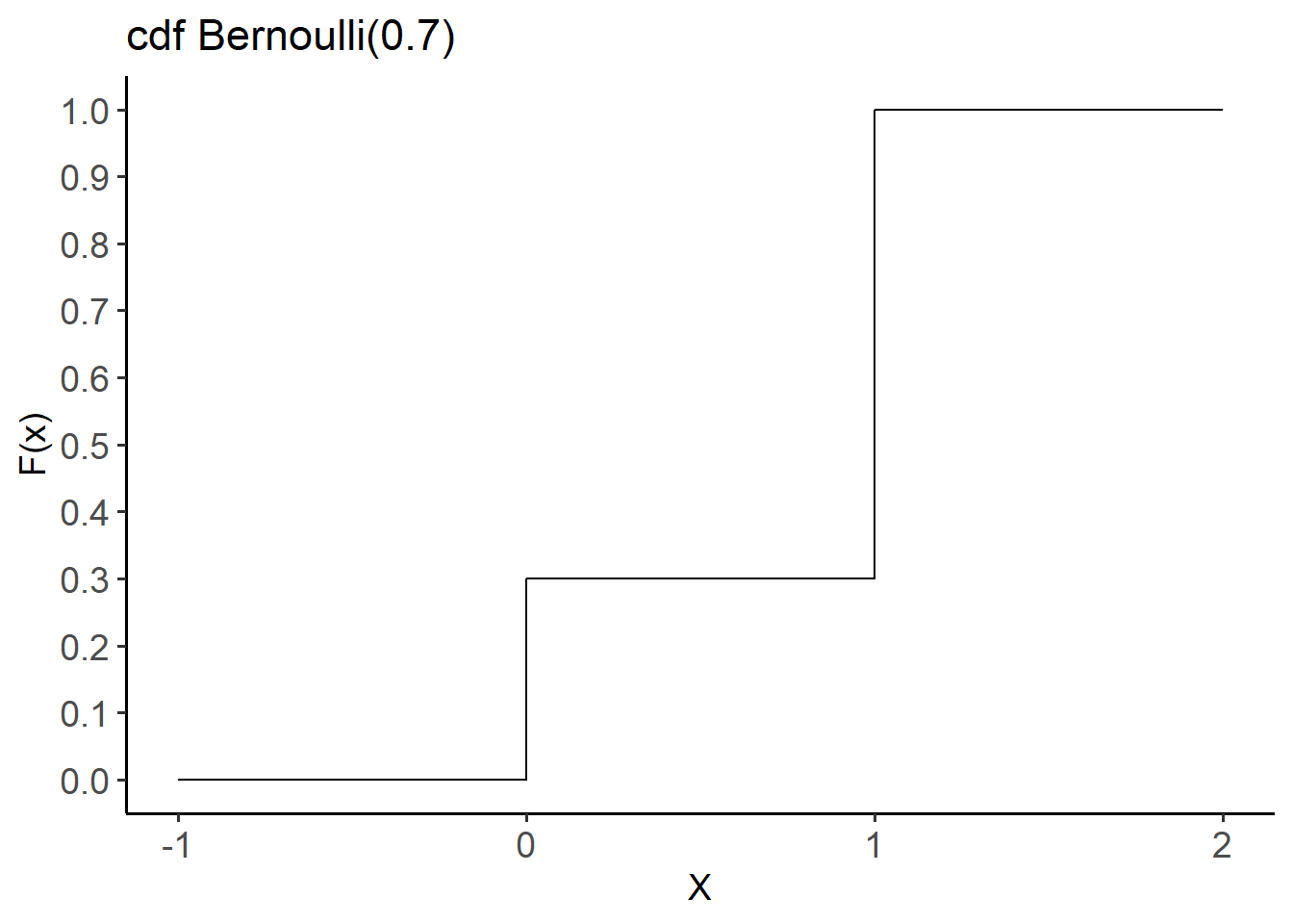

Figure 14.3: Plot of the cdf for Bernoulli(0.7) distribution.

 

• The mean is \(\mu\) = p = 0.7 and the variance is \(\sigma^2\) = 0.7(1-0.7)= 0.7\(\cdot\) 0.3 = 0.21.

14.3.2 Binomial distribution

The binomial probability distribution can be used for modeling the number of times a particular event occurs (successes) in a sequence of n repeated and independent Bernoulli trials, each with probability p of success.

The binomial setting

1. There is a fixed number of n repeated Bernoulli trials.
2. The n trials are all independent. That is, knowing the result of one trial does not change the probability we assign to other trials.
3. Both probability of success, p, and probability of failure, 1-p, are constant throughtout the trials.

Let X be a random variable that indicates the number of successes in n-independent Bernoulli trials. If random variable X satisfies the binomial setting, it follows the binomial distribution with parameters n and p, denoted as \(X ∼ Binomial(n, p)\), where n is the Bernoulli trial parameter (a positive integer) and p the Bernoulli probability parameter (\({0\leq p\leq 1}\)).

• The probability mass function (pmf) of X is given by:

\[ P(X=x) = {{n}\choose{x}} \cdot p^x \cdot (1-p)^{n-x} \tag{14.10}\]

where x = 0, 1, … , n and \(\binom{n}{x} = \frac{n!}{x!(n-x)!}\)

Note that: \(n! = 1\cdot 2 \cdot 3\cdot \ldots \cdot (n-2)\cdot (n-1)\cdot n\)

 

• The cumulative distribution function (cdf) of X is given by:

\[F(x) = P(X \le x)= {\begin{cases}0,&for\ x <0\\\sum_{k=0}^{x}{\left( \begin{array}{c} n \\ k \end{array} \right) p^{k}(1 - p)^{n-k}},&for\ 0\leq x < n\\1,&for\ x \geq n \end{cases}} \tag{14.11}\]

 

The mean of random variable, X, with Binomial(n, p) distribution is:

\[μ = np \tag{14.12}\]

the variance is:

\[σ^2 = np(1-p) \tag{14.13}\]

and the standard deviation:

\[σ = \sqrt{np(1-p)} \tag{14.14}\]

 

  Example

Let the random variable X be the number of successful surgical procedures and suppose that a new surgery method is successful 70% of the time (p = 0.7). If the results of 10 surgeries are randomly sampled, and X follows a Binomial distribution \(X ∼ Binomial(10, 0.7)\), find the main characteristics of this distribution.

• So, the pmf for this distribution is:

\[ P(X=x) = {{10}\choose{x}} \cdot 0.7^x \cdot (1-0.7)^{10-x} \tag{14.15}\]

The pmf of Binomial(10, 0.7) distribution specifies the probability of 0 through 10 successful surgical procedures.

According to Equation 14.15 we have:

Table 14.1: Probability table for \(X ∼ Poisson(2.5)\).

X	0	1	2	3	…	8	9	10
P(X)	0	0.0001	0.0014	0.009	…	0.233	0.121	0.028

We can easily compute the above probabilities using the dbinom() function in R:

dbinom(0:10, size = 10, prob = 0.7)

 [1] 0.0000059049 0.0001377810 0.0014467005 0.0090016920 0.0367569090
 [6] 0.1029193452 0.2001209490 0.2668279320 0.2334744405 0.1210608210
[11] 0.0282475249

We can plot the pmf for visualizing the distribution (Figure 14.4).

# Create a data frame
dat3 <- data.frame(x = 0:10, 
                   y = dbinom(0:10, size = 10, prob = 0.7))

# Plot
ggplot(dat3, aes(x = x, y = y)) +
  geom_segment(aes(x = x, xend=x, y=0, yend = y), color = "black") +
  geom_point(color="deeppink", size = 4) +
  theme_classic(base_size = 14) +
  scale_x_continuous(limits = c(0, 10), breaks = seq(0, 10, 1)) +
  labs(title = "pmf Binomial(10, 0.7)",
       x = "X", y = "Probability") +
  theme(axis.text = element_text(size = 14))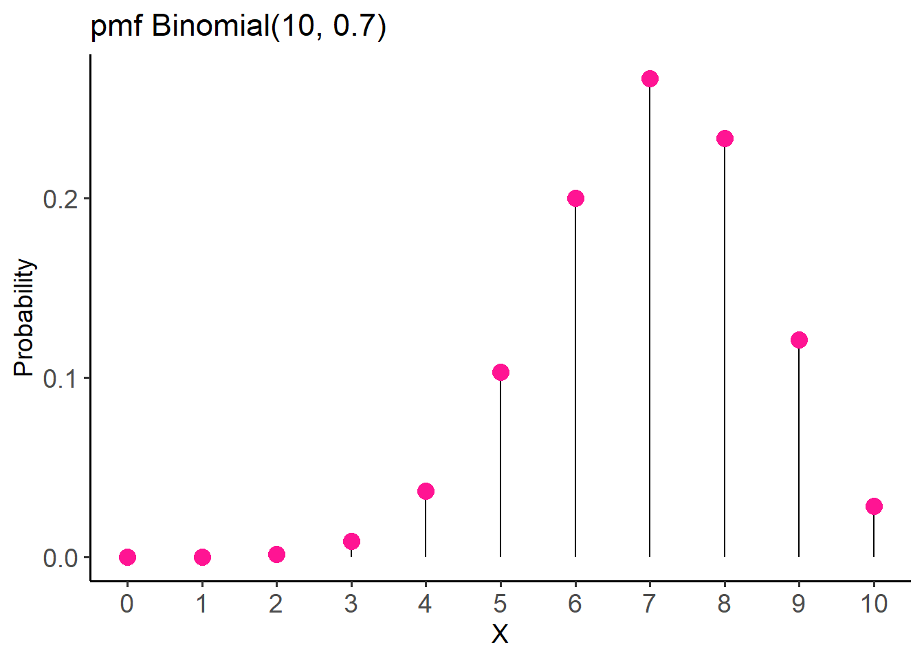

Figure 14.4: Plot of the pmf for Binomial(10, 0.7) distribution.

• The cdf for this distribution is:

\[F(x) = P(X \le x)={\begin{cases}0,&for\ x <0\\\sum_{k=0}^{x}{\left( \begin{array}{c} 10 \\ k \end{array} \right) 0.7^{k}(1 - 0.7)^{10-k}},&for\ 0\leq x < 10\\1,&for\ x \geq 10 \end{cases}} \tag{14.16}\]

In R, we can calculate the cumulative probabilities for all the possible outcomes using the pbinom() as follows:

# find the cumulative probabilities
pbinom(0:10, size = 10, prob = 0.7)

 [1] 0.0000059049 0.0001436859 0.0015903864 0.0105920784 0.0473489874
 [6] 0.1502683326 0.3503892816 0.6172172136 0.8506916541 0.9717524751
[11] 1.0000000000

The cdf for this distribution is shown below (Figure 14.5):

# Create a data frame
dat4 <- data.frame(x = 0:10, 
                   y = pbinom(0:10, size = 10, prob = 0.7))

# Step line plot
ggplot(dat4, aes(x=x, y=y)) +
  geom_step() +
  theme_classic(base_size = 14) +
  scale_x_continuous(limits = c(0, 10), breaks = seq(0, 10, 1)) +
  scale_y_continuous(limits = c(0, 1), breaks = seq(0, 1, 0.1)) +
  labs(title = "cdf Binomial(10, 0.7)",
       x = "X", y = "F(x)") +
  theme(axis.text = element_text(size = 14))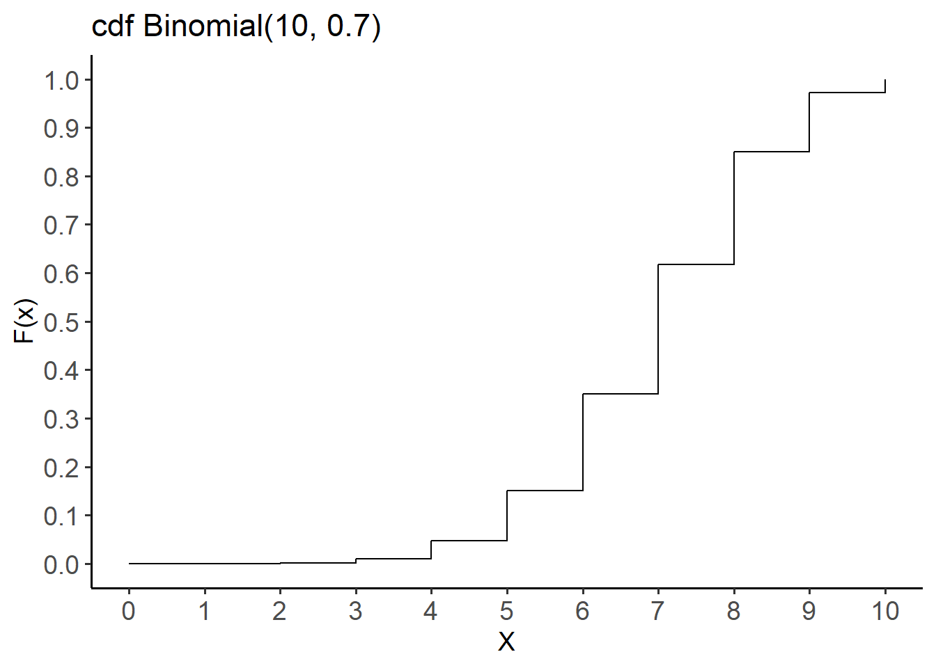

Figure 14.5: Plot of the cdf for Binomial(10, 0.7) distribution.

 

• The mean is \(\mu\) = n p = 10 \(\cdot\) 0.7 = 7 successful surgeries and the variance is \(\sigma^2\) = n p (1-p) = 10 \(\cdot\) 0.7 \(\cdot\) 0.3 = 2.1

Let’s calculate the probability of having having more than 8 successful surgical procedures out of a total of 10. Therefore, we want to calculate the probability P(X > 8):

\[ P(X > 8)= P(X = 9) + P(X = 10) = {{10}\choose{9}} \cdot 0.7^9 \cdot 0.3^1 + {{10}\choose{10}} \cdot 0.7^{10} \cdot 0.3^0 \Rightarrow \]

\[ P(X > 8)= 10 \cdot 0.04035 \cdot 0.3 + 1 \cdot 0.02824 = 0.12105 + 0.02825 = 0.1493\]

In R, we can calculate the probabilities P(X = 9) and P(X = 10) by applying the function dbinom() and adding the results:

p9 <- dbinom(9, size=10, prob=0.7)
p9

[1] 0.1210608

p10 <- dbinom(10, size=10, prob=0.7)
p10

[1] 0.02824752

p9 + p10

[1] 0.1493083

Of note, another way to find the above probability is to calculate the 1-P(X ≤ 8):

1 - pbinom(8, size=10, prob=0.7)

[1] 0.1493083

14.3.3 Poisson distribution

While a random variable with a Binomial distribution describes a count variable (e.g., number of successful surgeries), its range is restricted to whole numbers from 0 to n. For example, in a set of 10 surgical procedures (n = 10), the number of successful surgeries cannot surpass 10.

Now, let’s suppose that we are are interested in the number of successful surgeries per month in a particular specialty within a hospital. Theoretically, in this case, it is possible for the values to extend indefinitely without a predetermined upper limit.

Therefore, using the Poisson distribution, we can estimate the probability of observing a certain number of successful surgeries in a given month.

The Poisson setting

1. The events (occurrences) are counted within a fixed interval of time or space. The interval should be well-defined and consistent.
2. Each event is assumed to be independent of the others. The occurrence of one event does not affect the probability of another event happening.
3. The probability of an event occurring remains consistent throughout the interval.

Let X be a random variable that indicates the number of events (occurrences) that happen within a fixed interval of time or space. If \(λ\) represents the average rate of events (occurrences) in this interval or space, the X has a Poisson distribution that is specified by the parameter \(λ\), denoted as \(X ∼ Poisson(λ)\), where \(λ\) is a positive real number (\(λ >0\)).

• The probability mass function (pmf) of X is given by:

\[ P(X=x)={\frac {\lambda ^{x}e^{-\lambda }}{x!}} \tag{14.17}\]

where x = 0, 1, … +∞, λ > 0.

• The cumulative distribution function (cdf) of X is given by:

\[F(x) = P(X \le x)= {\begin{cases}0,&for\ x <0\\\sum_{k=0}^{x}{ \begin{array}{c} \frac {\lambda ^{k}e^{-\lambda }}{k!} \end{array}},&for\ x\geq 0 \end{cases}} \tag{14.18}\]

The mean and variance of a random variable that follows the Poisson(λ) distribution are the same and equal to λ:

• μ = λ
• \(σ^2\) = λ

  Example

Let X be a random variable of the number of successful heart transplant surgeries per week in a specialized cardiac center. We assume that the average rate of successful surgeries per week is 2.5 (\(λ = 2.5\)), and X follows a Poisson distribution: \(X ∼ Poisson(2.5)\)

• According to Equation 14.17, the probability mass function (pmf) of X is:

\[ P(X=x)={\frac {2.5 ^{x}e^{-2.5 }}{x!}} \]

The resulting probability table is:

Table 14.2: Probability table for \(X ∼ Poisson(2.5)\).

X	0	1	2	3	4	5	6	7	8	…
P(X)	0.082	0.205	0.257	0.214	0.134	0.067	0.028	0.01	0.003	…

We can compute the above probabilities using the dpois() function in R:

dpois(0:8, lambda = 2.5)

[1] 0.082084999 0.205212497 0.256515621 0.213763017 0.133601886 0.066800943
[7] 0.027833726 0.009940617 0.003106443

We can also plot the pmf for visualizing the distribution (Figure 14.6).

# Create a data frame
dat5 <- data.frame(x = 0:8, 
                   y = dpois(0:8, lambda = 2.5))

# Plot
ggplot(dat5, aes(x = x, y = y)) +
  geom_segment(aes(x = x, xend=x, y=0, yend = y), color = "black") +
  geom_point(color="deeppink", size = 4) +
  theme_classic(base_size = 14) +
  scale_x_continuous(limits = c(0, 8), breaks = seq(0, 8, 1)) +
  labs(title = "pmf Poisson(2.5)",
       x = "X", y = "Probability") +
  theme(axis.text = element_text(size = 14))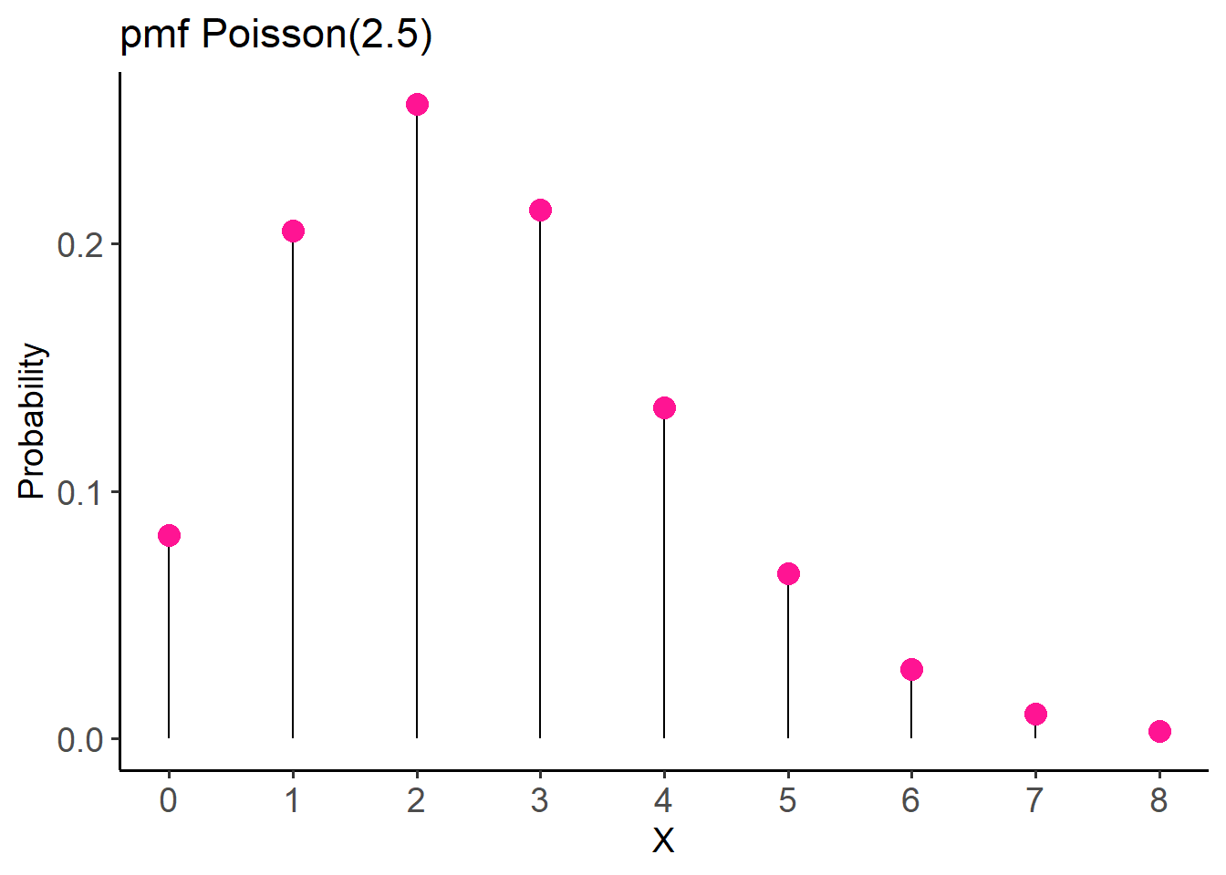

Figure 14.6: Plot of the pmf for Poisson(2.5) distribution.

For this example, the probability of none successful heart transplant surgery in a week is P(X = 0) = 0.08, while the probability of exactly two successful surgeries per week increases to P(X = 2) = 0.257.

 

• In R, we can calculate the cumulative probabilities for all the possible outcomes using the ppois() as follows:

# find the cumulative probabilities
ppois(0:8, lambda = 2.5)

[1] 0.0820850 0.2872975 0.5438131 0.7575761 0.8911780 0.9579790 0.9858127
[8] 0.9957533 0.9988597

The cdf for this distribution is shown below (Figure 14.7):

# Create a data frame
dat6 <- data.frame(x = 0:8, 
                   y = ppois(0:8, lambda = 2.5))

# Step line plot
ggplot(dat6, aes(x=x, y=y)) +
  geom_step() +
  theme_classic(base_size = 14) +
  scale_x_continuous(limits = c(0, 8), breaks = seq(0, 8, 1)) +
  scale_y_continuous(limits = c(0, 1), breaks = seq(0, 1, 0.1)) +
  labs(title = "cdf Poisson(2.5)",
       x = "X", y = "F(x)") +
  theme(axis.text = element_text(size = 14))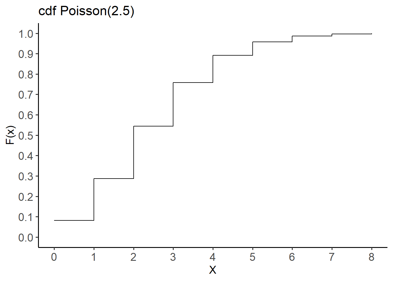

Figure 14.7: Plot of the pmf for Poisson(2.5) distribution.

 

• The mean and variance of this variable are \(\mu\)= 2.5 and \(\sigma^2\) = 2.5, respectively.

Let’s calculate the probability of up to four successful heart transplant surgeries per week. Therefore, we want to calculate the cumulative probability \(P(X \le 4)= \sum_{k=0}^4 \frac {\lambda ^{k}e^{-\lambda }}{k!}\). In practice, we can add the individual probabilities from the Table 14.2 for the corresponding outcomes:

P(X ≤ 4) = P(X = 0) + P(X = 1) + P(X = 2) + P(X = 3) + P(X = 4) = 0.082 + 0.205 + 0.257 + 0.214 + 0.134 = 0.892.

In R, we can calculate this probability by applying the function ppois():

ppois(4, lambda = 2.5)

[1] 0.891178

So, the probability of up to four successful heart transplant surgeries per week in the specialized cardiac center is approximately 0.89 or 89%.

14.4 Probability distributions for continuous outcomes

Unlike discrete random variables, which have a probability mass function (pmf) that assigns probabilities to individual values, continuous random variables have a probability density function (pdf), denoted as f(x), which satisfies the following properties:

• \(f(x) \geq 0\)
• \(\int_{-\infty}^{+\infty} f(x) \, dx = 1\)

In this case, we are interested in the probability that the value of the random variable X is within a specific interval from \(x_1\) to \(x_2\), denoted as \(P(x_1 ≤ X ≤ x_2)\).

\[ P(x_1\leq X \leq x_2)=\int_{x_1}^{x_2}f(x)dx \tag{14.19}\]

The graphical representation of the probability density function referred to as a density plot (Figure 14.8). In this plot, the x-axis represents the possible values of the variable X, while the y-axis represents the probability density.

# Create a data frame
set.seed(1234)
df <- data.frame(w = round(c(rnorm(200, mean=175, sd=8),
                             rnorm(200, mean=155, sd=8)))
                 )

df1 <- with(density(df$w), data.frame(x, y))

ggplot(df1, mapping = aes(x = x, y = y)) +
  geom_line()+
  geom_area(mapping = aes(x = ifelse(x > 170 & x < 175 , x, 0)), fill = "#0073CF") +
  xlim(120, 210) +
  labs(y = "f(x)") +
  scale_y_continuous(expand = c(0,0)) +
  theme_classic(base_size = 14)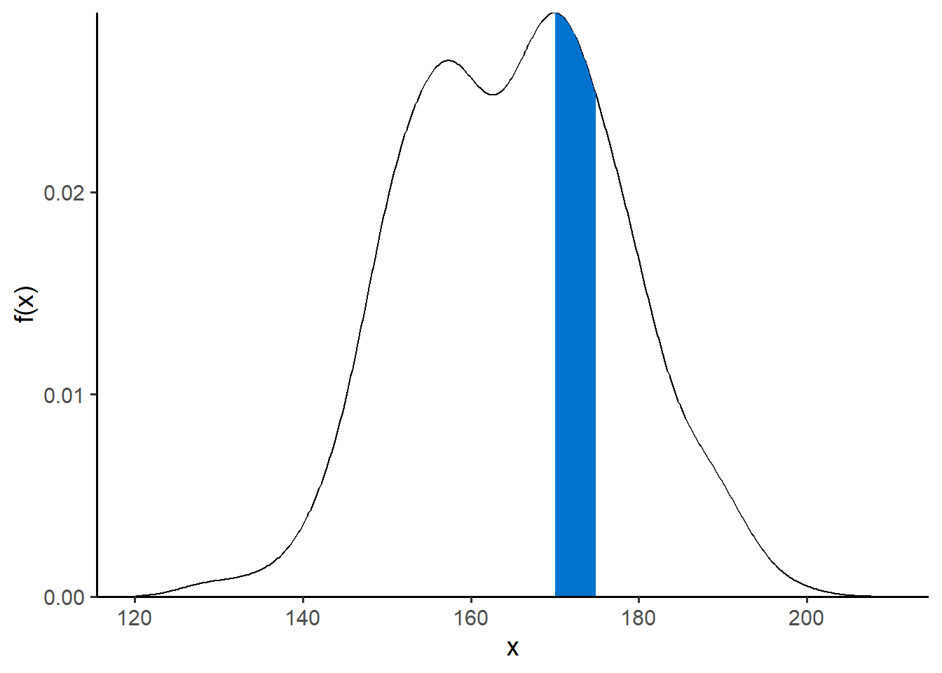

Figure 14.8: Density plot.

Additionally, from the pdf we can find the cumulative probability by calculating the area from -∞ to a specific value \(x_o\) (shaded blue area in Figure 14.9). The cumulative distribution function (cdf) gives the probability that the random variable X is less than or equal to \(x_o\) and is usually denoted as:

\[ F(x_o) = P(X\leq x_o)=\int_{- \infty }^{x_o}f(x)dx \tag{14.20}\] where \(-\infty \leq x_o \leq + \infty\)

ggplot(df1, mapping = aes(x = x, y = y)) +
  geom_line()+
  geom_area(mapping = aes(x = ifelse(x > -Inf & x < 173 , x, 0)), fill = "#0073CF") +
  xlim(120, 210) +
  labs(y = "f(x)") +
  scale_y_continuous(expand = c(0,0)) +
  theme_classic(base_size = 14)

Figure 14.9: Plot of the cumulative probability.

Note

The probability of a certain point value in X is zero, and the area under the probability density curve of the interval (−∞, +∞) should be 1.

The expected value, variance, and standard deviation for a continuous random variable X are as follows:

Expected Value

The expected value or mean, denoted as E(X) or μ, is calculated by integrating over the entire range of possible values:

\(\mu =E(X) = \int_{-\infty}^{+\infty} x \cdot f(x) \, dx\)

Variance

We can also calculate the variance of the variable X.

\(\sigma^2=\text{Var}(X) = E[(X - \mu)^2] = \int_{-\infty}^{+\infty} (x - \mu)^2 \cdot f(x) \, dx\)

Standard deviation

The standard deviation is often preferred over the variance because it is in the same units as the random variable.

\(\sigma=\sqrt{\text{Var(X)}}=\sqrt{\sigma^2}\)

14.4.1 Uniform distribution

The simplest continuous probability distribution is the uniform distribution.
Let X be a continuous random variable that follows the uniform distribution with parameters the minimum value \(a\) and the maximum value \(b\) (\(a < b\)), \(X ∼ Uniform(\alpha,b)\)

• The probability density function (pdf) of X is given by:

\[f(x) = \begin{cases} \frac{1}{b - a} & \text{for } a \leq x \leq b \\ 0 & \text{otherwise} \end{cases} \tag{14.21}\]

• The cumulative distribution function (cdf) of X is:

\[F(x) = \begin{cases} 0 & \text{for } x < a \\ \frac{x - a}{b - a} & \text{for } a \leq x \leq b \\ 1 & \text{for } x > b \end{cases} \tag{14.22}\]

The mean of X is given by:

\[\mu = \frac{a + b}{2}\]

The variance of the X is given by: \[\sigma^2 = \frac{(b - a)^2}{12}\]

The uniform distribution, with a=0 and b=1, is highly useful as a random number generator. Let’s see an example of simple randomization in a clinical trial.

 

  Example

Let X be a random variable that follows the uniform distribution Uniform(0, 1). Find the main characteristics of this distribution.

Then utilize this distribution to randomize 100 individuals between treatments A and B in a clinical trial.

NOTE: The simple randomization with the Uniform(0,1) distribution ensures that each individual in the study has an equal chance of being assigned to either treatment group.

• The pdf for this distribution is:

\[f(x) = \begin{cases} 1 & \text{for } 0 \leq x \leq 1 \\ 0 & \text{otherwise} \end{cases}\]

# Define the range of x values (including values outside the range)
x_values <- seq(-0.5, 1.5, by = 0.01)

# Calculate the PDF values for the uniform distribution
pdf_values <- dunif(x_values, min = 0, max = 1)

# Create a data frame for the PDF plot
pdf_data <- data.frame(x = x_values, PDF = pdf_values)

# Plot the PDF
ggplot(pdf_data, aes(x = x, y = PDF)) +
  geom_line() +
  xlim(-0.5, 1.5) +
  labs(title = "pdf Uniform(0, 1)",
       x = "X", y = "P(x)") +
  theme(axis.text = element_text(size = 14))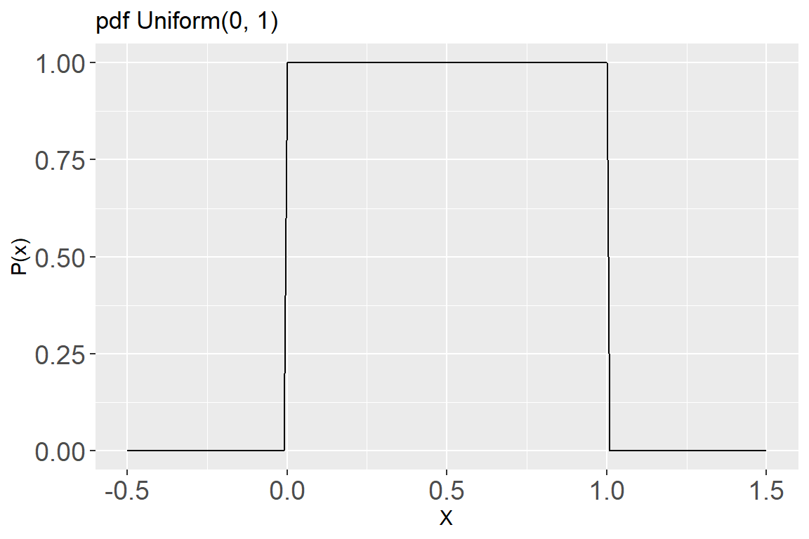

Figure 14.10: Plot of the pdf for Uniform(0, 1) distribution.

• The cdf for this distribution is:

\[F(x) = \begin{cases} 0 & \text{for } x < 0 \\ x & \text{for } 0 \leq x \leq 1 \\ 1 & \text{for } x > 1 \end{cases} \]

# Calculate the CDF values for the uniform distribution
cdf_values <- punif(x_values, min = 0, max = 1)

# Create a data frame for the CDF plot
cdf_data <- data.frame(x = x_values, CDF = cdf_values)

# Plot the CDF
ggplot(cdf_data, aes(x = x, y = CDF)) +
  geom_line() +
  xlim(-0.5, 1.5) +
    labs(title = "cdf Uniform(0, 1)",
         x = "X", y = "F(x)") +
  theme(axis.text = element_text(size = 14))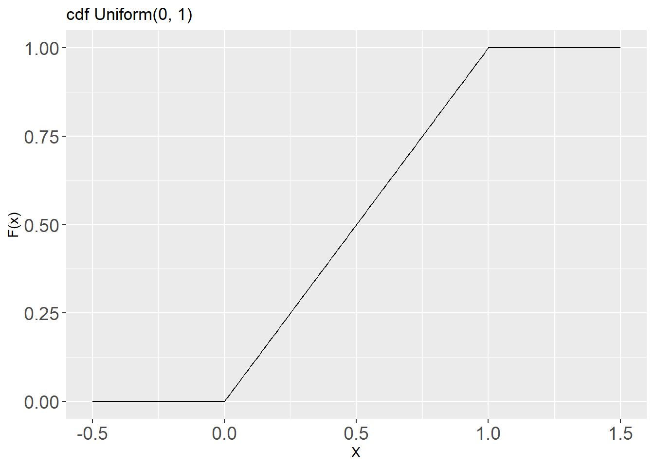

Figure 14.11: Plot of the cdf for Poisson(2.5) distribution.

The mean and variance of a random variable that follows the Uniform(0, 1) distribution are:

• \(μ = \frac{0 + 1}{2} = \frac{1}{2}\)
• \(σ^2 = \frac{(1 - 0)^2}{12} = \frac{1}{12}\)

Next, we use the Uniform(0, 1) to randomize individuals between treatments A and B in a clinical trial:

# Set seed for reproducibility
set.seed(235)

# Define the sample size of the clinical trial
N <- 100

# Create a data frame to store the information
data <- data.frame(id = paste("id", 1:N, sep = ""), trt = NA)

# Simulate 100 uniform random variables from (0-1)
x <- runif(N)
# Display the first 10 values
x[1:10]

 [1] 0.98373365 0.79328881 0.60725184 0.12093957 0.24990178 0.52147467
 [7] 0.96265857 0.92370588 0.45026693 0.07862284

# Make treatment assignments, if x < 0.5 treatment A else B
data$trt <- ifelse(x < 0.5, "A", "B")

# Display the first few rows of the data frame
head(data, 10)

     id trt
1   id1   B
2   id2   B
3   id3   B
4   id4   A
5   id5   A
6   id6   B
7   id7   B
8   id8   B
9   id9   A
10 id10   A

# Display the counts and proportions of each treatment
table(data$trt)

 A  B 
48 52 

prop.table(table(data$trt))

   A    B 
0.48 0.52 

14.4.2 Normal distribution

A normal distribution, also known as a Gaussian distribution, is a fundamental concept in statistics and probability theory and is defined by two parameters: the mean (μ) and the standard deviation (σ) (see Chapter 15).

• The probability density function (pdf) of \(X ∼ Normal(μ, σ^2)\) is given by:

\[ f(x)={\frac {1}{\sigma {\sqrt {2\pi }}}}e^{-{\frac {1}{2}}\left({\frac {x-\mu }{\sigma }}\right)^{2}} \tag{14.23}\]

where \(\pi \approx 3.14\) and \(e \approx 2.718\).

• The cumulative distribution function (cdf) of X sums from negative infinity up to the value of \(x_o\), which is \((-∞, x_o]\) in interval notation:

\[ F(x_o) = P(X\leq x_o)={\frac {1}{\sigma {\sqrt {2\pi }}}} \int_{- \infty }^{x_o}e^{-{\frac {1}{2}}\left({\frac {x-\mu }{\sigma }}\right)^{2}}dx \tag{14.24}\] where \(-\infty \leq x_o \leq + \infty\)

  Example

Let’s say that in a population the random variable of height, X, for adult people approximates a normal distribution with a mean μ = 170 cm and a standard deviation σ = 10 cm.

The pdf for this distribution is shown below (Figure 14.12):

ggplot() +
  geom_function(fun = dnorm, args = list(mean = 170, sd = 10), 
                color= "gray20", linewidth = 1) +
  xlim(135, 205) +
  labs(x = "X", y = "Probabiblity Density, f(x)",
       title = "The Normal Distribution, N~(170, 10^2)") +
  scale_y_continuous(expand = c(0,0)) +
  theme_classic(base_size = 14)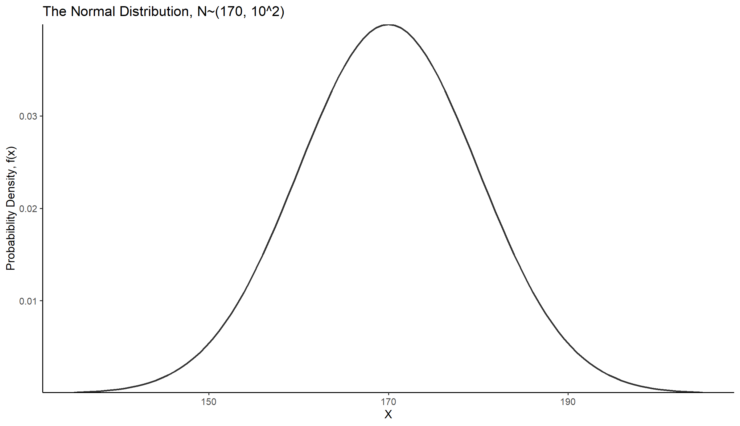

Figure 14.12: The Normal Distribution

The Figure 14.13 illustrates the normal cumulative distribution function. Note that continuous variables generate a smooth curve, while discrete variables produce a stepped line plot.

# Create a data frame
dat7 <- data.frame(x = seq(135, 205, by = 0.1), 
                   y = pnorm(seq(135, 205, by = 0.1), mean=170, sd=10))
# Plot
ggplot(dat7, aes(x=x, y=y)) +
  geom_step() +
  labs(x = "X", y = "Cumulative Probabiblity, F(x)") +
  scale_y_continuous(expand = c(0,0)) +
  theme_classic(base_size = 14)

Figure 14.13: The normal cumulative distribution function.

 

Let’s assume that we want to calculate the area under the curve between 160 cm and 180 cm, that is:

\[ P(160\leq X \leq 180)=\int_{160}^{180}f(x)dx \]

# Create a data frame
df2 <- data.frame(x = seq(135, 205, by = 0.1),
                   y = dnorm(seq(135, 205, by = 0.1), mean=170, sd=10))

# Create the plot
ggplot(df2, aes(x = x, y = y)) +
  geom_function(fun = dnorm, args = list(mean = 170, sd = 10), 
                color= "gray20", linewidth = 1) +
  geom_area(mapping = aes(x = ifelse(x > 160 & x < 180, x, 0)), fill = "#0073CF", alpha = 0.4) +  # Area under the curve
  xlim(135, 205) +
  labs(x ="x", y = "Probability density",
       title = "Area Under the Normal Distribution Curve") +
  scale_y_continuous(expand = c(0,0)) +
  theme_classic(base_size = 14)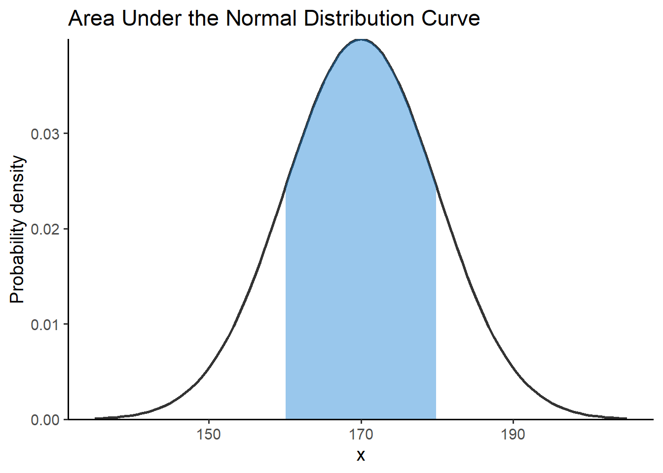

Figure 14.14: Plot of the distribution.

Using the properties of integrals we have:

\[ \int_{-\infty}^{180}f(x)dx = \int_{-\infty}^{160}f(x)dx + \int_{160}^{180}f(x)dx \] \[ \Leftrightarrow \int_{160}^{180}f(x)dx = \int_{-\infty}^{180}f(x)dx - \int_{-\infty}^{160}f(x)dx \] \[ \Leftrightarrow P(160\leq X \leq 180) = P(X \leq 180)- P(X \leq 160) \]

Therefore, one way to find the area under the curve between 160 cm and 180 cm is to calculate the cdf at each of these values and then find the difference between them:

• Lets calculate the \(P(X \leq 180)\):

\[ P(X \leq 180)=\int_{-\infty}^{180}f(x)dx \]

# Create the plot
ggplot(df2, aes(x = x, y = y)) +
  geom_function(fun = dnorm, args = list(mean = 170, sd = 10), 
                color= "gray20", linewidth = 1) +
  geom_area(mapping = aes(x = ifelse(x > 135 & x < 180, x, 0)), fill = "#0073CF", alpha = 0.4) +  # Area under the curve
  xlim(135, 200) +
  labs(x = "X", y = "Probability density",
       title = "Area Under the Normal Distribution Curve") +
  scale_y_continuous(expand = c(0,0)) +
  theme_classic(base_size = 14)

Figure 14.15: Plot of the distribution.

pnorm(180, mean = 170, sd = 10)

[1] 0.8413447

 

• Similarly, we can calculate the \(P(X \leq 160)\):

\[ P(X \leq 160)=\int_{-\infty}^{160}f(x)dx \]

# Create the plot
ggplot(df2, aes(x = x, y = y)) +
  geom_function(fun = dnorm, args = list(mean = 170, sd = 10), 
                color= "gray20", linewidth = 1) +
  geom_area(mapping = aes(x = ifelse(x > 135 & x < 160, x, 0)), fill = "#0073CF", alpha = 0.3) +  # Area under the curve
  xlim(135, 200) +
  labs(x = "X", y = "Probability density",
       title = "Area Under the Normal Distribution Curve") +
  scale_y_continuous(expand = c(0,0)) +
  theme_classic(base_size = 14)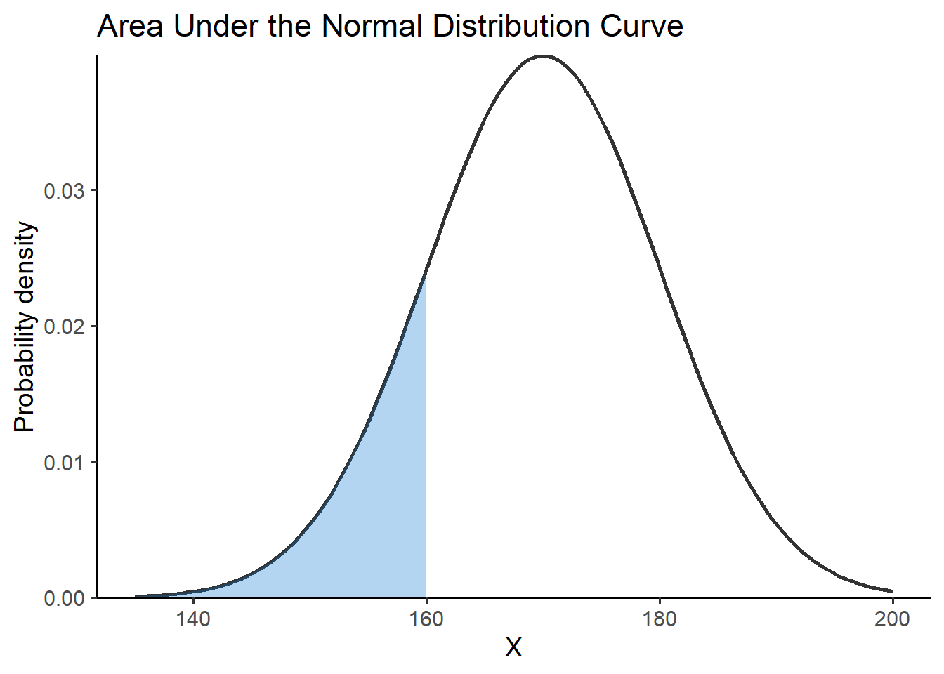

Figure 14.16: Plot of the distribution.

pnorm(160, mean = 170, sd = 10)

[1] 0.1586553

 

Finally, we subtract the two values (shaded blue areas) as follows:

pnorm(180, mean = 170, sd = 10) - pnorm(160, mean = 170, sd = 10)

[1] 0.6826895

14.4.3 Standard Normal distribution

If X is a random variable with a normal distribution having a mean of \(\mu\) and a standard deviation of \(\sigma\), then the standardized Normal deviate can be expressed as:

\[ z= \frac{x-\mu}{\sigma} \tag{14.25}\]

The z (often called z-score) is a random variable that has a Standard Normal distribution, also called a z-distribution, i.e. a special normal distribution where \(\mu=0\) and \(\sigma^2=1\). In this case, Equation 14.23 is transformed as follows:

\[ f(z)={\frac {1}{{\sqrt {2\pi }}}}e^{-{\frac {1}{2}}z^2} \tag{14.26}\]

ggplot() +
  stat_function(fun = dnorm, args = list(mean = 0, sd = 1)) +
  scale_x_continuous(limits = c(-3, 3), breaks = seq(-3, 3, 1)) +
  labs(x = "Z", y = "Probabiblity density, f(z)",
       title = "The Standard Normal Distribution, N~(0, 1^2)") +
  scale_y_continuous(expand = c(0,0.005)) +
  theme_classic(base_size = 14)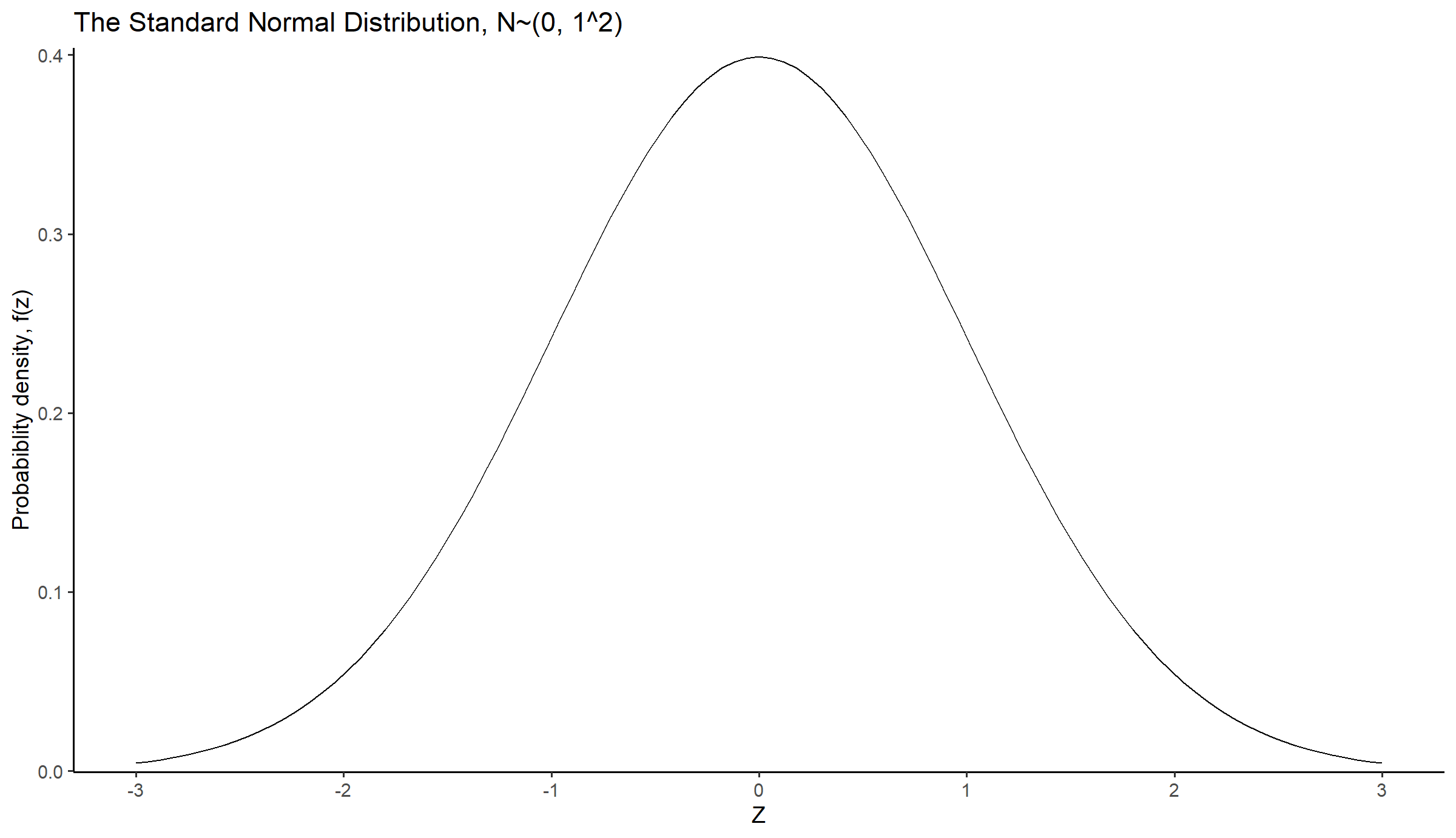

Figure 14.17: The Standard Normal Distribution

Z-scores are commonly used in medical settings to assess how an individual’s measurement compares to the average value of the entire population.

  Example

Let’s assume that the diastolic blood pressure distribution among men has a normal distribution with mean 80 mmHg and standard deviation 15 mmHg. If an individual’s diastolic blood pressure is recorded as 110 mmHg, how many standard deviations differs from the population mean?

The z-score Equation 14.25 is:

\(z = \frac{(110 – 80)}{15} = 2\)

So this person has a diastolic blood pressure that is 2 standard deviations above the population mean.

To find the area under the curve between two z-scores, \(z_1\) and \(z_2\), we have to integrate the pdf Equation 14.26 as follows:

\[ P(z_1\leq Z\leq z_2)={\frac {1}{{\sqrt {2\pi }}}}\int_{z_1}^{z_2}e^{-{\frac {1}{2}}z^2}dz \tag{14.27}\]

For example, let’s calculate the area under the curve in Figure 14.18, for \(z_1\) = 0 and \(z_2\) = 2:

# Create a data frame
df3 <- data.frame(x = seq(-3, 3, by = 0.01),
                   y = dnorm(seq(-3, 3, by = 0.01), mean=0, sd=1))

ggplot(df3, aes(x = x, y = y)) +
  stat_function(fun = dnorm, args = list(mean = 0, sd = 1)) +
  geom_area(mapping = aes(x = ifelse(x > 0 & x < 2, x, 0)), fill = "#0073CF", alpha = 0.3) +  # Area under the curve
  scale_x_continuous(limits = c(-3, 3), breaks = seq(-3, 3, 1)) +
  labs(x = "Z", y = "Probabiblity density, f(z)",
       title = "The Standard Normal Distribution, N~(0, 1^2)") +
  scale_y_continuous(expand = c(0,0)) +
  theme_classic(base_size = 14)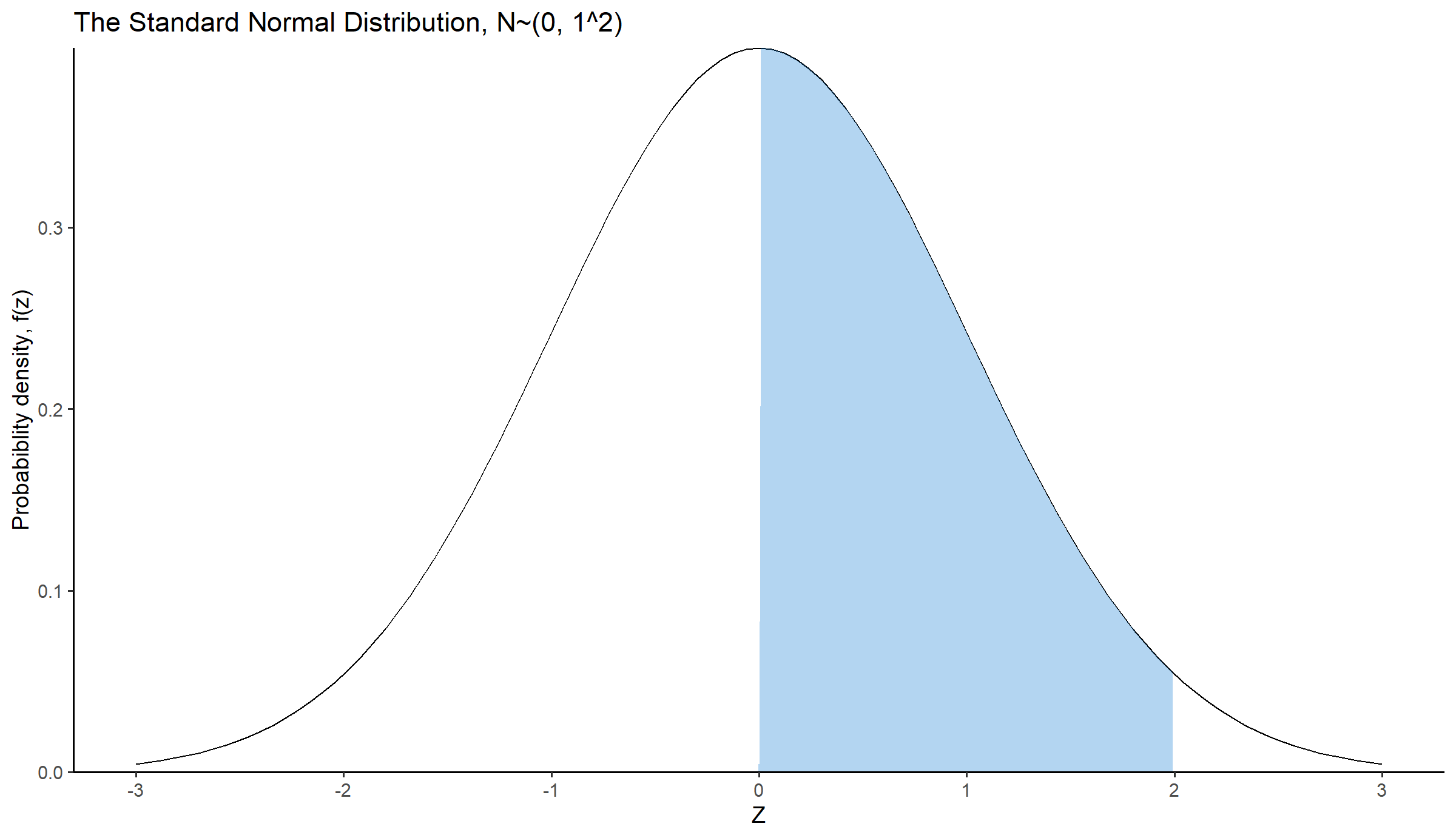

Figure 14.18: The Standard Normal Distribution

In R, we can easily calculate the above area using the cdf of the normal distribution:

\[P(0\leq Z\leq 2) = P(Z\leq 2) - P(Z\leq 0)\]

pnorm(2, mean = 0, sd = 1) - pnorm(0, mean = 0, sd = 1)

[1] 0.4772499

14.4.4 Chi-square distribution

The chi-square distribution arises in various contexts, such as the chi-square test for independence in Chapter 30.

Let \(Z_1, Z_2,..., Z_{\nu}\) be independent random variables that follow the standard normal distribution N(0,1). Then, the sum of the squares of these standard normal random variables, \(U=\sum_{i=1}^n Z_i^2\), follows the chi-squared distribution with \(\nu\) degrees of freedom, \(U \sim\chi_\nu^2\).

Therefore, the chi-squared distribution is determined by a single parameter, \(\nu\), which specifies the degrees of freedom (the number of random variables Z being summed). For example, the square of a standard normal variable follows the chi-square distribution with one degree of freedom, \(U = Z_{1}^2 \sim \chi_1^2\).

The mean and variance of a random variable that follows the chi-square distribution with \(\nu\) degrees of freedom are:

• \(μ = \nu\)
• \(σ^2 = 2\nu\)

The shape of the chi-square distribution depends on the degrees of freedom, \(\nu\).

ggplot(data = data.frame(x = c(0, 20)), aes(x = x)) +
  stat_function(fun = function(x) dchisq(x, df = 3), aes(color = "Chi-square (df = 3)"), size = 0.8) +
  stat_function(fun = function(x) dchisq(x, df = 5), aes(color = "Chi-square (df = 5)"), size = 0.8) +
  stat_function(fun = function(x) dchisq(x, df = 9), aes(color = "Chi-square (df = 9)"), size = 0.8) +
  scale_x_continuous(limits = c(0, 20), breaks = seq(0, 20, 1)) +
  scale_color_manual(values = c("purple", "orange", "cyan"),
                     labels = c("ν = 3", "ν = 5", "ν = 9")) +
  labs(x = "Chi-square", y = "Probability Density") +
  scale_y_continuous(expand = c(0,0)) +
  theme_classic(base_size = 14) +
  theme(legend.title = element_blank())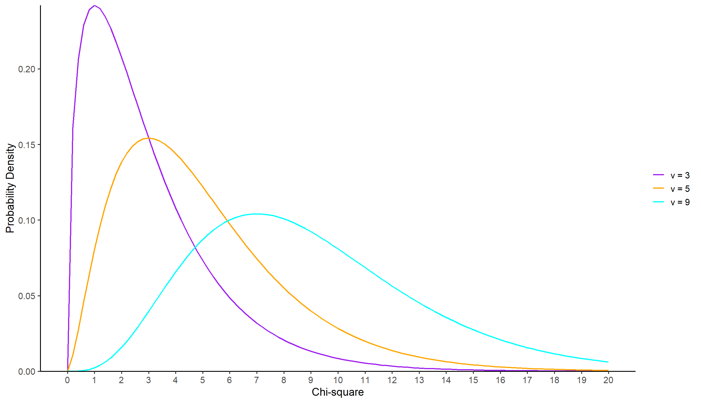

Figure 14.19: Family of chi-Square distributions

NOTE: When \(\nu\) is large, the shape of the chi-square distribution becomes increasingly similar to that of a normal distribution.

14.4.5 t-distribution

The t-distribution, also known as the Student’s t-distribution, is very similar to standard normal distribution and is used in statistics when the sample size is small or when the population standard deviation is unknown.

The Student’s t statistic is defined from the formula:

\[ T = \frac{Z}{\sqrt\frac{{U}}{\nu}} \]

where Z∼N(0,1) and U∼\(\chi_\nu^2\) are independent.

The t statistic follows the t-distribution with \(\nu\) degrees of freedom. As the degrees of freedom increase (\(\nu\)> 30), the t-distribution approaches the normal distribution more closely.

The mean and variance of a random variable that follows the t-distribution with \(\nu\) degrees of freedom are:

• \(\mu= 0\), \(\nu \geq 2\)
• \(σ^2 = \nu/(\nu −2)\) , \(\nu \geq 3\)

The shape of the t-distribution depends on the degrees of freedom, \(\nu\) (Figure 14.20).

ggplot(data = data.frame(x = c(-5, 5)), aes(x = x)) +
  stat_function(fun = dnorm, args = list(mean = 0, sd = 1), aes(color = "a"), size = 0.8) +
  stat_function(fun = function(x) dt(x, df = 3), aes(color = "b = 3"), size = 0.8) +
  stat_function(fun = function(x) dt(x, df = 5), aes(color = "c = 5"), size = 0.8) +
  stat_function(fun = function(x) dt(x, df = 9), aes(color = "d = 9"), size = 0.8) +
  scale_x_continuous(limits = c(-5, 5), breaks = seq(-5, 5, 1)) +
  scale_color_manual(values = c("black", "purple", "orange", "cyan"),
                     labels = c("Standard Normal", "ν = 3", "ν = 5", "ν = 9")) +
  labs(x = "t", y = "Probabiblity Density") +
  scale_y_continuous(expand = c(0,0)) +
  theme_classic(base_size = 14) +
  theme(legend.title = element_blank())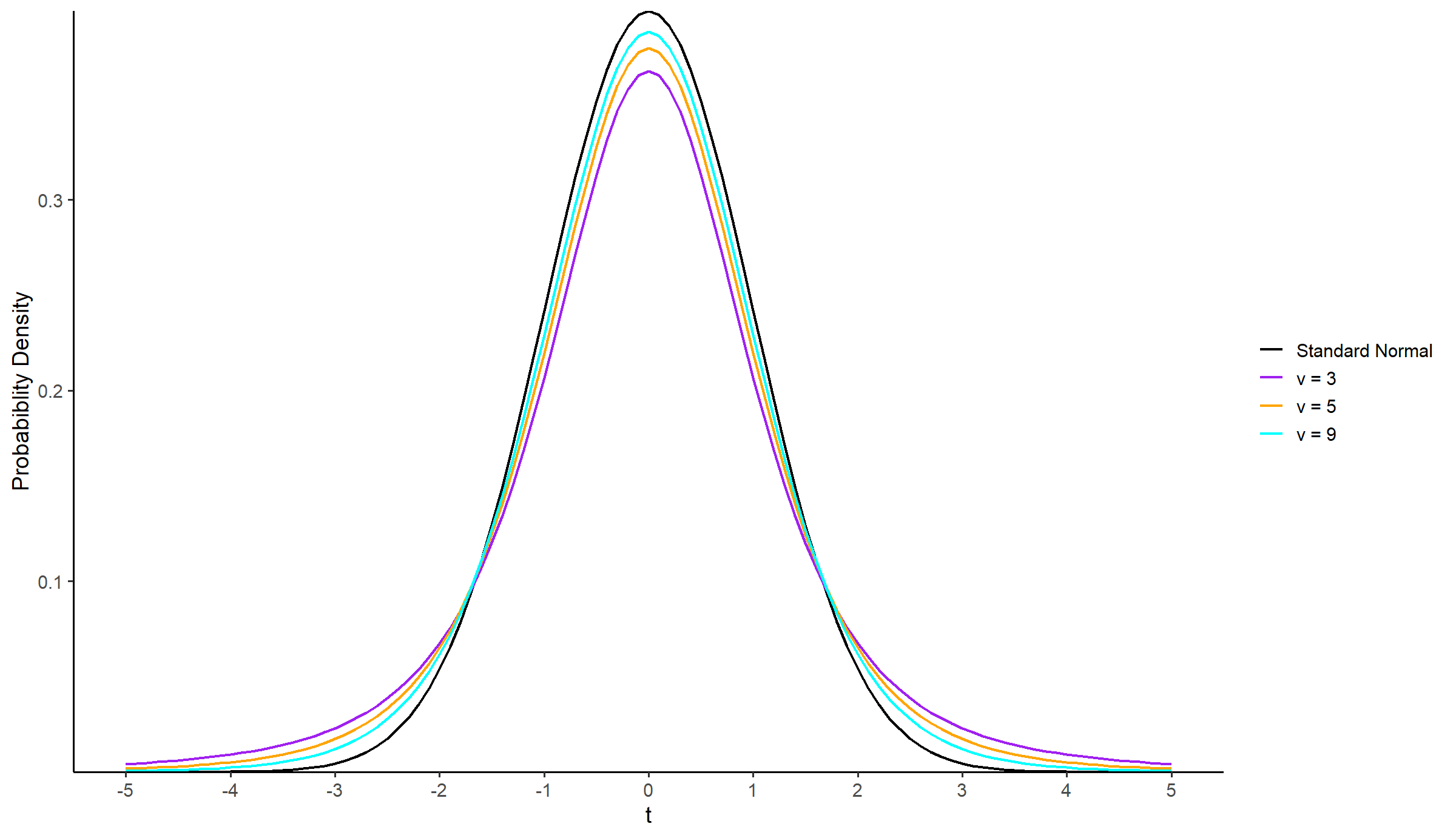

Figure 14.20: t-distribution family with ν=3, 5, 9 Vs Standard Normal distribution

Just like the standard normal distribution, the probability density curve of a t-distribution is bell-shaped and symmetric around its mean (μ = 0). However, the probability density curve of the t-distribution decreases more slowly than that of the standard normal distribution (t-distribution has “heavier” tails than the standard normal distribution).

If the area of the curve is known, it is possible to calculate the corresponding t-value. For example, in Figure 14.21, if each of the shaded light blue areas equal to 0.025, we can find the t-value using the qt() function in R:

# Create a data frame
df4 <- data.frame(x = seq(-5, 5, by = 0.01),
                  y = dt(seq(-5, 5, by = 0.01), df = 3))

ggplot() +
  stat_function(fun = dnorm, args = list(mean = 0, sd = 1)) +
  stat_function(fun = dt, args = list(df = 3), color  = "purple") +
  geom_area(data = df4, mapping = aes(x = ifelse(x < -3, x, -3), y = y), fill = "#0073CF", alpha = 0.3) +  # Area under the curve
  geom_area(data = df4, mapping = aes(x = ifelse(x > 3, x, 3), y = y), fill = "#0073CF", alpha = 0.3) +  # Area under the curve
  scale_x_continuous(limits = c(-5, 5), breaks = seq(-5, 5, 1)) +
  annotate("text", x = 0, y = 0.41, label = "standard normal") +
  annotate("text", x = 0, y = 0.38, label = "t(3)", color = "purple") +
  labs(x = "t", y = "Probabiblity Density") +
  scale_y_continuous(expand = c(0,0)) +
  theme_classic(base_size = 14)

Figure 14.21: t-distribution with df=3 Vs Standard Normal distribution

qt(0.025, df = 3)

[1] -3.182446

qt(0.975, df = 3)

[1] 3.182446

14.4.6 F-distribution

Let U and V be independent random variables that follow the \(\chi_{\nu_1}^2\) and \(\chi_{\nu_2}^2\), respectively. Then, the random variable:

\[F = \frac{U / \nu_1}{V / \nu_2} \]

follows the F-distribution with \(\nu_1\) and \(\nu_2\) degrees of freedom, \(F \sim F_{\nu_1, \nu_2}\).

The shape of an F-distribution depends on the values of \(\nu_1\) and \(\nu_2\), the numerator and denominator degrees of freedom, respectively (Figure 14.22):

ggplot(data = data.frame(x = c(0, 5)), aes(x = x)) +
  stat_function(fun = function(x) df(x, df1 = 2, df2 = 1), aes(color = "v1 = 2, v2 = 1"), size = 0.8) +
  stat_function(fun = function(x) df(x, df1 = 3, df2 = 5), aes(color = "v1 = 3, v2 = 5"), size = 0.8) +
  stat_function(fun = function(x) df(x, df1 = 10, df2 = 8), aes(color = "v1 = 10, v2 = 8"), size = 0.8) +
  scale_x_continuous(limits = c(0, 5), breaks = seq(0, 5, 1)) +
  scale_color_manual(values = c("purple", "orange", "cyan"),
                     labels = c("v1 = 2, v2 = 1", "v1 = 3, v2 = 5", "v1 = 10, v2 = 8")) +
  labs(x = "F", y = "Probability Density") +
  scale_y_continuous(expand = c(0,0)) +
  theme_classic(base_size = 14) +
  theme(legend.title = element_blank())

Figure 14.22: F-distribution family

The mean and variance of a random variable that follows the F-distribution with \(\nu_1\) and \(\nu_2\) degrees of freedom are:

• \(\mu = \frac{\nu_2}{\nu_2 - 2}\)

• \(\sigma^2 = \frac{2 \nu_2^2 (\nu_1 + \nu_2 - 2)}{\nu_1 (\nu_2 - 2)^2 (\nu_2 - 4)}\)