10  Data import, pre-processing, and transformation

This chapter focuses on importing data from spreadsheets into R and covers essential techniques for manipulating, transforming, and summarizing data effectively. We also introduce the powerful native forward pipe operator |>, which streamlines the process by allowing operations to be chained together in a clear and concise manner. Additionally, we present and explain the process of reshaping data between wide and long formats in R.

# Required packages for this chapter
library(readxl)              
library(janitor)             
library(here) 
library(tidyverse)

 

10.1 Importing data

Spreadsheets are commonly used to organize structured, rectangular data and are available in formats such as Excel, CSV, or Google Sheets. Each format offers unique features, from Excel’s comprehensive capabilities to CSV’s simplicity and Google Sheets’ collaborative editing. In this textbook, most datasets are provided in Excel files (.xlsx) and typically have the following basic characteristics:

• The first line in the file is a header row, specifying the names of the columns (variables).
• Each value has its own cell.
• Missing values are represented as empty cells.

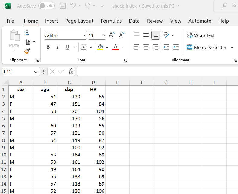
For example, FIGURE 10.1 shows a screenshot of data from a single sheet of an Excel file. The dataset, named shock_index, contains information about the characteristics of 30 adult patients suspected of having a pulmonary embolism. The following variables were recorded:

• sex: F for females and M for males
• Age: age of the patients in years
• SBP: systolic blood pressure in mmHg
• HR: resting heart rate in beats/min

FIGURE 10.1 Screenshot of an Excel file.

10.1.1 Importing data from Excel using the RStudio Interface

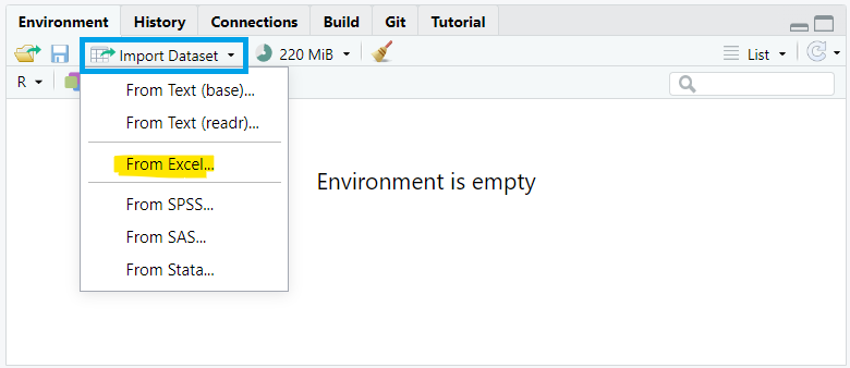
To import data using the RStudio interface, we navigate to the Environment pane, where we’ll find the “Import Dataset” button. Clicking this button will prompt a dropdown menu with options to import data from various file formats such as CSV, Excel, or other common formats. We select “From Excel…” (FIGURE 10.2).

FIGURE 10.2 Importing data using the RStudio interface.

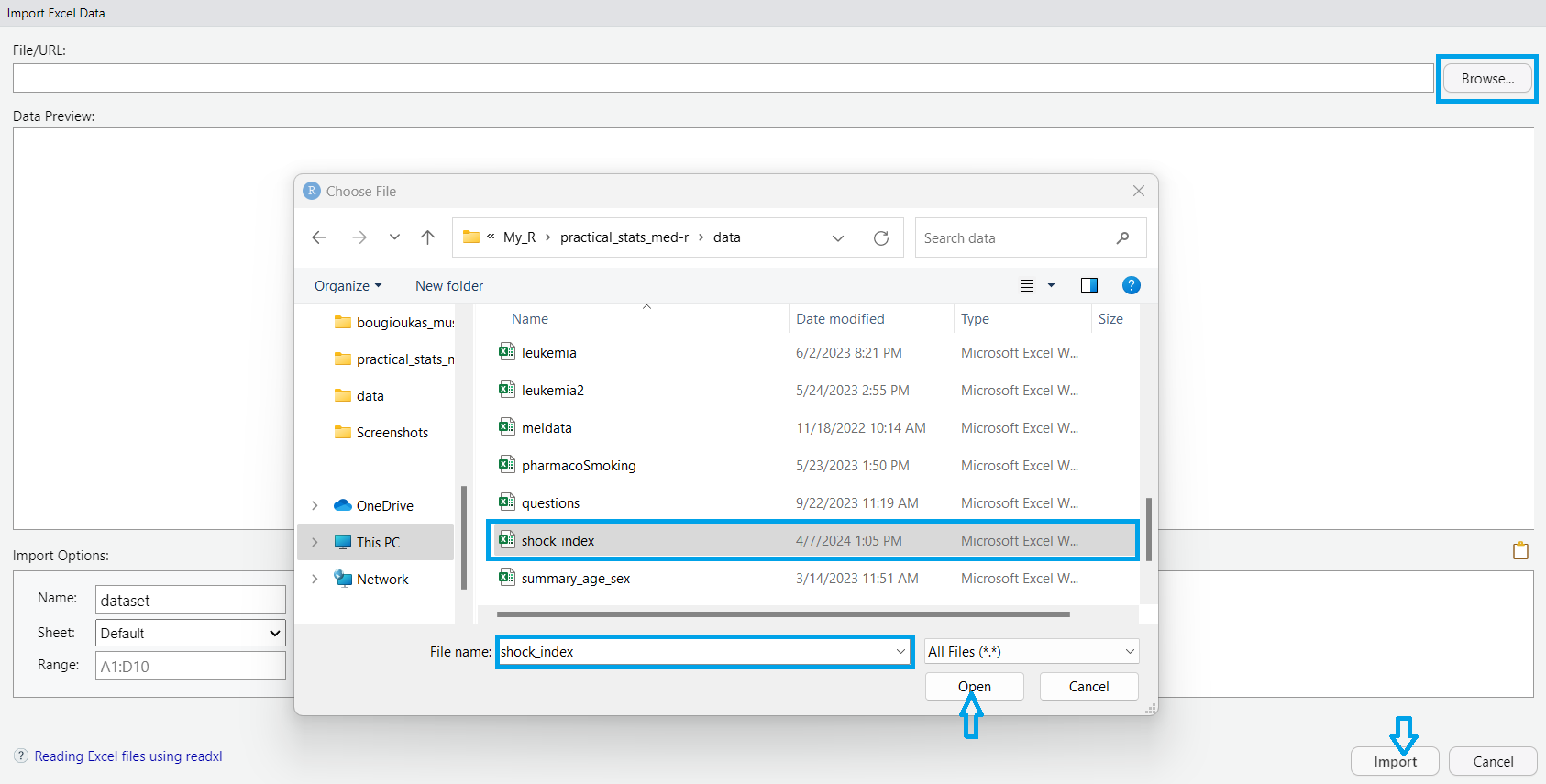
A dialog box then appears, enabling us to navigate our file system and specify the desired dataset (FIGURE 10.3). Once selected, we confirm the import by clicking “Open”. Finally, we proceed by clicking the “Import” button, which imports the selected dataset into our RStudio session.”

FIGURE 10.3 Specifying the dataset for import.

After a successful import, the dataset will be displayed in the Environment pane, allowing for further manipulation.

10.1.2 Importing data from Excel into R with commands

Alternatively, if the dataset is saved in the subfolder named “data” of our RStudio project (see also Chapter 2), we can read it with the read_excel() function from readxl package as follows:

dat <- read_excel(here("data", "shock_index.xlsx"))

The path of a file (directory) is its location in the file system (address). As we have previously discussed, there are two kinds of paths.

• absolute paths such as “C:/My_name/../my_project/data/shock_index.xlsx” and
• relative paths such as “data/shock_index.xlsx”.

The function here() allows us to navigate throughout each of the subfolders and files within a given RStudio Project using relative paths (see also Chapter 5).

Using head() is a convenient way to get a quick overview of our dataset and check for any obvious issues before proceeding with further analysis or data manipulation.

head(dat)

# A tibble: 6 × 4
  sex     Age   SBP    HR
  <chr> <dbl> <dbl> <dbl>
1 M        54   139    85
2 F        47   151    84
3 F        58   200   100
4 M        NA   170    56
5 F        60   123    55
6 F        57   121    90

By default, the first six rows of the data frame are displayed. To view a different number of rows (e.g., the first ten), we can specify the desired number as an argument, like this: head(dat, 10).

Additionally, when working with large datasets in R, it’s often useful to inspect the last few rows of a data frame. The tail() function is used for this purpose:

tail(dat)

# A tibble: 6 × 4
  sex     Age   SBP    HR
  <chr> <dbl> <dbl> <dbl>
1 M        58   119    87
2 F        48   104    93
3 F        55   164    69
4 M        59    92   119
5 F        48   127   109
6 F        51   136    60

Now, the last six rows of the data frame are displayed in the R console.

10.2 Pre-processing data

10.2.1 Adding an unique identifier for each observation

A unique identifier for each observation is often useful for various data manipulation and analysis tasks. In R, we can add row numbers starting from 1 to the number of rows in our data frame using the rowid_to_column() function from the tibble package:

dat <- rowid_to_column(dat)
head(dat)

# A tibble: 6 × 5
  rowid sex     Age   SBP    HR
  <int> <chr> <dbl> <dbl> <dbl>
1     1 M        54   139    85
2     2 F        47   151    84
3     3 F        58   200   100
4     4 M        NA   170    56
5     5 F        60   123    55
6     6 F        57   121    90

10.2.2 Renaming variables and cleaning names

Choosing informative column names can significantly enhance the clarity and interpretability of our dataset. For instance, renaming rowid to patient_ID clarifies that this column serves as a unique identifier for each patient. Likewise, renaming HR to Heart.Rate offers a more intuitive and informative label for the heart rate variable.

dat <- rename(dat, 
               patient_ID = rowid,
               Heart.Rate = HR)
head(dat)

# A tibble: 6 × 5
  patient_ID sex     Age   SBP Heart.Rate
       <int> <chr> <dbl> <dbl>      <dbl>
1          1 M        54   139         85
2          2 F        47   151         84
3          3 F        58   200        100
4          4 M        NA   170         56
5          5 F        60   123         55
6          6 F        57   121         90

However, it’s crucial to ensure that the column names are consistent with the naming conventions in R. This can be achieved by using the clean_names() function from the janitor package, which standardizes column names by converting them to lowercase, removing special characters, and replacing spaces with underscores.

dat <- clean_names(dat)
head(dat)

# A tibble: 6 × 5
  patient_id sex     age   sbp heart_rate
       <int> <chr> <dbl> <dbl>      <dbl>
1          1 M        54   139         85
2          2 F        47   151         84
3          3 F        58   200        100
4          4 M        NA   170         56
5          5 F        60   123         55
6          6 F        57   121         90

10.2.3 Converting to the appropriate data type

We might have noticed that the categorical variable sex is coded as F (for females) and M (for males), so it is recognized of character type. We can use the factor() function to encode a variable as a factor:

dat$sex <- factor(dat$sex, levels = c("F", "M"), labels = c("female", "male"))
head(dat)

# A tibble: 6 × 5
  patient_id sex      age   sbp heart_rate
       <int> <fct>  <dbl> <dbl>      <dbl>
1          1 male      54   139         85
2          2 female    47   151         84
3          3 female    58   200        100
4          4 male      NA   170         56
5          5 female    60   123         55
6          6 female    57   121         90

10.2.4 Handling missing values

Upon reviewing the dataset, it’s apparent that there are missing values in the age variable, denoted as NA. Various techniques exist to handle missing values in data such as excluding observations with any missing values, substituting with a constant value (mean, median, mode), or employing multiple imputation methods. The choice of method depends on factors such as the proportion of missing data, its distribution, and understanding the underlying mechanism behind the missingness (whether it’s random or non-random) (Altman and Bland 2007; Heymans and Twisk 2022).

While this introductory textbook primarily uses datasets without missing values, it’s important to note that missing data present a frequent challenge in real-world data analysis. Fortunately, several R packages are tailored to address this issue, including: mice, VIM, naniar, and Hmisc.

 

10.3 Transforming data

10.3.1 Subsetting observations (rows)

Subsetting observations (rows) is a common data manipulation task in data analysis, allowing us to focus on specific subsets of data that meet particular criteria. This process involves selecting rows from a dataset based on conditions we specify.

10.3.1.1 Select observations by indexing position within [ ]

Just as we use square brackets [row, column] to select elements from matrices, we apply the same approach to select elements from a data frame. For example, by specifying the row indices [5:10, ] within the brackets, we can select the data for rows 5 through 10:

dat1 <- dat[5:10, ]
dat1

# A tibble: 6 × 5
  patient_id sex      age   sbp heart_rate
       <int> <fct>  <dbl> <dbl>      <dbl>
1          5 female    60   123         55
2          6 female    57   121         90
3          7 male      54   120         84
4          8 male      NA   100         92
5          9 female    53   164         72
6         10 male      58   161        102

10.3.1.2 Select observations by using logical conditions inside [ ]

By applying logical conditions, such as greater than (>), less than (<), equal to (==), or combinations of these, we can filter observations that meet specific criteria.

• For example, we can filter the data to find patients whose age is greater than 55, as follows:

dat2 <- dat[dat$age > 55, ]
dat2

# A tibble: 13 × 5
   patient_id sex      age   sbp heart_rate
        <int> <fct>  <dbl> <dbl>      <dbl>
 1          3 female    58   200        100
 2         NA <NA>      NA    NA         NA
 3          5 female    60   123         55
 4          6 female    57   121         90
 5         NA <NA>      NA    NA         NA
 6         10 male      58   161        102
 7         13 female    57   118         89
 8         17 male      56   126        107
 9         19 male      59   138         85
10         20 male      56   153         85
11         24 female    57   121         90
12         25 male      58   119         87
13         28 male      59    92        119

Step-by-step explanation: First, the code evaluates the expression dat$age > 55 for each row in the data frame, generating a logical vector where TRUE indicates patients older than 55 and FALSE indicates others. This logical vector is then used inside the square brackets [ ] to subset the data frame, selecting only the rows where the condition is TRUE. The resulting subset is assigned to the new object dat2. Note that when there are missing values in the age column, the corresponding rows in dat2 contain NA values.

Similarly, we can use the which() function that returns the indices where the condition age > 55 is TRUE. However, in this case, the missing values are treated as FALSE, resulting in the exclusion of rows where age in the original data is NA.

dat3 <- dat[which(dat$age > 55), ]
dat3

# A tibble: 11 × 5
   patient_id sex      age   sbp heart_rate
        <int> <fct>  <dbl> <dbl>      <dbl>
 1          3 female    58   200        100
 2          5 female    60   123         55
 3          6 female    57   121         90
 4         10 male      58   161        102
 5         13 female    57   118         89
 6         17 male      56   126        107
 7         19 male      59   138         85
 8         20 male      56   153         85
 9         24 female    57   121         90
10         25 male      58   119         87
11         28 male      59    92        119

• If our objective is to analyze data for female patients aged over 55, we can create a subset by incorporating the logical & operator to combine the conditions for age and sex.

dat4 <- dat[which(dat$age > 55 & dat$sex == "female"), ]
dat4

# A tibble: 5 × 5
  patient_id sex      age   sbp heart_rate
       <int> <fct>  <dbl> <dbl>      <dbl>
1          3 female    58   200        100
2          5 female    60   123         55
3          6 female    57   121         90
4         13 female    57   118         89
5         24 female    57   121         90

The resulting data frame contains only the rows that meet both of these conditions, namely females over 55 years old.

10.3.1.3 Select observations using the filter() function from dplyr

The dplyr package also provides the filter() function for selecting observations.

• Selecting rows where age is greater than 55:

dat5 <- filter(dat, age > 55)
dat5

# A tibble: 11 × 5
   patient_id sex      age   sbp heart_rate
        <int> <fct>  <dbl> <dbl>      <dbl>
 1          3 female    58   200        100
 2          5 female    60   123         55
 3          6 female    57   121         90
 4         10 male      58   161        102
 5         13 female    57   118         89
 6         17 male      56   126        107
 7         19 male      59   138         85
 8         20 male      56   153         85
 9         24 female    57   121         90
10         25 male      58   119         87
11         28 male      59    92        119

• Selecting rows where age is greater than 55 and patient is female:

dat6 <- filter(dat, age > 55 & sex == "female")
dat6

# A tibble: 5 × 5
  patient_id sex      age   sbp heart_rate
       <int> <fct>  <dbl> <dbl>      <dbl>
1          3 female    58   200        100
2          5 female    60   123         55
3          6 female    57   121         90
4         13 female    57   118         89
5         24 female    57   121         90

The above code is equivalent to the following command:

filter(dat, age > 55, sex == "female")

IMPORTANT

When multiple logical expressions are separated by a comma within the filter() function, they are effectively combined using the & operator.

 

10.3.2 Reordering observations (rows)

Another useful data manipulation involves sorting observations in ascending or descending order of one or more variables (columns). When multiple column names are provided, each additional column helps resolve ties in preceding columns’ values.

• For example, to arrange the rows of our data based on the values of sbp in ascending order (the default), we can run the following code:

dat7 <- arrange(dat, sbp)
head(dat7)

# A tibble: 6 × 5
  patient_id sex      age   sbp heart_rate
       <int> <fct>  <dbl> <dbl>      <dbl>
1         16 male      48    92        122
2         28 male      59    92        119
3          8 male      NA   100         92
4         26 female    48   104         93
5         15 female    50   109        142
6         13 female    57   118         89

• To rearrange the data in descending order based on sbp, we can use the desc() function within the arrange() function:

dat8 <- arrange(dat, desc(sbp))
head(dat8)

# A tibble: 6 × 5
  patient_id sex      age   sbp heart_rate
       <int> <fct>  <dbl> <dbl>      <dbl>
1         21 male      48   201        104
2          3 female    58   200        100
3          4 male      NA   170         56
4         22 female    52   170         57
5          9 female    53   164         72
6         11 female    49   164         90

The above code is equivalent to the following command:

arrange(dat, -sbp)  # The minus sign indicates descending order

• We can also sort the data in ascending (or descending) order based first on the values in the column sbp and then on the values in the column heart_rate.

dat9 <- arrange(dat, sbp, heart_rate)
head(dat9)

# A tibble: 6 × 5
  patient_id sex      age   sbp heart_rate
       <int> <fct>  <dbl> <dbl>      <dbl>
1         28 male      59    92        119
2         16 male      48    92        122
3          8 male      NA   100         92
4         26 female    48   104         93
5         15 female    50   109        142
6         13 female    57   118         89

Notably, two patients (IDs 16 and 28) share the lowest systolic blood pressure of 92 mmHg. When sorting in ascending order, if multiple patients have the same systolic blood pressure, these observations are further sorted by heart rate, with lower heart rate taking precedence. In this case, patient 28, with a heart rate of 119 beats/min, is listed before patient 16, whose heart rate is 122 beats/min.

10.3.3 Subsetting variables (columns)

When working with data frames, selecting specific variables (columns) for analysis is a common task. For instance, suppose we want to select only the sex, age, and heart_rate variables from the data frame.

10.3.3.1 Select variables by indexing their name within [ ]

Subsetting variables can be achieved by indexing the variables’ names within [ ], as follows:

dat10 <- dat[, c("sex", "age" , "heart_rate")]
head(dat10)

# A tibble: 6 × 3
  sex      age heart_rate
  <fct>  <dbl>      <dbl>
1 male      54         85
2 female    47         84
3 female    58        100
4 male      NA         56
5 female    60         55
6 female    57         90

10.3.3.2 Select variables by indexing position within [ ]

By specifying the column indices, such as c(2, 3, 5), within brackets, we can select the data in columns 2, 3, and 5 as follows:

dat11 <- dat[, c(2, 3, 5)]
head(dat11)

# A tibble: 6 × 3
  sex      age heart_rate
  <fct>  <dbl>      <dbl>
1 male      54         85
2 female    47         84
3 female    58        100
4 male      NA         56
5 female    60         55
6 female    57         90

Or we can exclude the variables in the first and forth position.

dat12 <- dat[-c(1, 4)]
head(dat12)

# A tibble: 6 × 3
  sex      age heart_rate
  <fct>  <dbl>      <dbl>
1 male      54         85
2 female    47         84
3 female    58        100
4 male      NA         56
5 female    60         55
6 female    57         90

10.3.3.3 Select variables using the select() function from dplyr

In select() function we pass the data frame first and then the variables separated by commas. Quotes are optional for column names that don’t contain special characters or spaces.

dat13 <- select(dat, sex, age, heart_rate)
head(dat13)

# A tibble: 6 × 3
  sex      age heart_rate
  <fct>  <dbl>      <dbl>
1 male      54         85
2 female    47         84
3 female    58        100
4 male      NA         56
5 female    60         55
6 female    57         90

Or we can exclude the variables patient_id and sbp.

select(dat, -c(patient_id, sbp))

# A tibble: 30 × 3
   sex      age heart_rate
   <fct>  <dbl>      <dbl>
 1 male      54         85
 2 female    47         84
 3 female    58        100
 4 male      NA         56
 5 female    60         55
 6 female    57         90
 7 male      54         84
 8 male      NA         92
 9 female    53         72
10 male      58        102
# ℹ 20 more rows

10.3.4 Creating new variables

Data analysis often involves creating new variables within data frames based on existing variables. This data transformation process involves adding new columns to a data frame derived from the values of one or more existing columns.

Suppose we want to compute a new variable representing the ratio of heart rate to systolic blood pressure (HR/sbp), which we will call shock_index. We can achieve this by using the mutate() function from dplyr package, as follows:

dat14 <- mutate(dat, shock_index = heart_rate / sbp)

head(dat14)

# A tibble: 6 × 6
  patient_id sex      age   sbp heart_rate shock_index
       <int> <fct>  <dbl> <dbl>      <dbl>       <dbl>
1          1 male      54   139         85       0.612
2          2 female    47   151         84       0.556
3          3 female    58   200        100       0.5  
4          4 male      NA   170         56       0.329
5          5 female    60   123         55       0.447
6          6 female    57   121         90       0.744

IMPORTANT

By default, the mutate() function adds the new variable as the last column in the tibble.

 

Our next step involves categorizing the newly created shock_index variable based on the defined normal range (0.5 to 0.7 beats/mmHg $\cdot$ min). This can be done using the case_when() function from the dplyr package.

dat15 <- mutate(dat14,
                shock_index1 = case_when(shock_index < 0.5 ~ "low",
                                         shock_index <= 0.7 ~ "normal",
                                         TRUE ~ "high"))
head(dat15)

# A tibble: 6 × 7
  patient_id sex      age   sbp heart_rate shock_index shock_index1
       <int> <fct>  <dbl> <dbl>      <dbl>       <dbl> <chr>       
1          1 male      54   139         85       0.612 normal      
2          2 female    47   151         84       0.556 normal      
3          3 female    58   200        100       0.5   normal      
4          4 male      NA   170         56       0.329 low         
5          5 female    60   123         55       0.447 low         
6          6 female    57   121         90       0.744 high        

However, it’s important to keep in mind that transforming continuous variables into categories may simplify interpretation, but it often results in information loss.

10.3.5 Using the native pipe operator in a sequence of commands

Given that each verb in dplyr specializes in a particular task, addressing complex queries often typically involves integrating several verbs, a process simplified by using the native forward pipe operator, |>.

For example, we want to filter the original dataset to include only rows where the shock index category is “low” or “high”, using a sequence of dplyr verbs.

sub_dat <- dat |>
  mutate(shock_index = heart_rate / sbp,
         shock_index1 = case_when(shock_index < 0.5 ~ "low",
                                  shock_index <= 0.7 ~ "normal",
                                  TRUE ~ "high")) |> 
  filter(shock_index1 == "low" | shock_index1 == "high")

We would read this sequence of commands as:

$\to$ Begin with the dataset dat, then

$\to$ Use it as input to the mutate() function to calculate the shock_index variable and create the shock_index1 categorical variable, then

$\to$ Use this output as input to the filter() function to select patients with “low” or “high” values of shock index.

The first six rows are shown below:

head(sub_dat)

# A tibble: 6 × 7
  patient_id sex      age   sbp heart_rate shock_index shock_index1
       <int> <fct>  <dbl> <dbl>      <dbl>       <dbl> <chr>       
1          4 male      NA   170         56       0.329 low         
2          5 female    60   123         55       0.447 low         
3          6 female    57   121         90       0.744 high        
4          8 male      NA   100         92       0.92  high        
5          9 female    53   164         72       0.439 low         
6         13 female    57   118         89       0.754 high        

Using the %in% operator inside the filter() function simplifies the code by enabling multiple logical OR conditions to be checked simultaneously.

dat |>
  mutate(shock_index = heart_rate / sbp,
         shock_index1 = case_when(shock_index < 0.5 ~ "low",
                                  shock_index <= 0.7 ~ "normal",
                                  TRUE ~ "high")) |>
  filter(shock_index1 %in% c("low", "high"))

INFO

The native forward pipe operator $|>$ was introduced in base R version 4.1.0. It provides a built-in way to chain function calls in R, similar to the functionality offered by the $>$ operator from the magrittr package.

 

10.4 Summarizing data

10.4.1 Summary measures

Let’s calculate two common summary measures of the age variable in our data frame: the sample mean and standard deviation. To compute these summary statistics, we use the mean() and sd() mathematical functions in R (Chapter 3).

mean(dat$age, na.rm = TRUE)

[1] 53.85714

sd(dat$age, na.rm = TRUE)

[1] 3.960119

Now, we’ll use the mean() and sd() within the summarize() generic function from the dplyr package. We’ll store the results in a new data frame called stats, which will contain two columns: the mean_age and the sd_age.

stats <- dat |> 
  summarize(mean_age = mean(age, na.rm = TRUE),
            sd_age = sd(age, na.rm = TRUE))
stats

# A tibble: 1 × 2
  mean_age sd_age
     <dbl>  <dbl>
1     53.9   3.96

INFO

The dplyr package also provides the alternative spelling summarise() for users who prefer the UK convention. Both functions work identically.

 

To calculate statistical summaries for multiple columns simultaneously, we can use the across() function within the summarize() function. For example:

dat |> 
  summarize(across(
    .cols = c(age, sbp),
    .fns = list(
      mean = \(x) mean(x, na.rm = TRUE),
      sd = \(x) sd(x, na.rm = TRUE)),
    .names = "{col}_{fn}")
)

# A tibble: 1 × 4
  age_mean age_sd sbp_mean sbp_sd
     <dbl>  <dbl>    <dbl>  <dbl>
1     53.9   3.96     137.   28.1

In the above syntax, the .cols argument specifies the columns to be summarized, while the .fns argument defines the functions to be applied, such as mean() and sd(), which are wrapped in a list. Finally, the .names argument specifies the naming convention for the output columns. Note that the expressions \(x) mean(x, na.rm = TRUE) and \(x) sd(x, na.rm = TRUE) are examples of “anonymous” functions in R and can also be written using the purrr-style lambda as ~ mean(.x, na.rm = TRUE) and ~ sd(.x, na.rm = TRUE), respectively.

dat |> 
  summarize(across(
    .cols = c(age, sbp),
    .fns = list(
      mean = ~ mean(.x, na.rm = TRUE),
      sd = ~ sd(.x, na.rm = TRUE)),
    .names = "{col}_{fn}")
)

INFO

Anonymous functions, also called lambda functions, are created “on-the-fly” in R without being assigned a name. They are commonly used within other functions or operations, providing a concise and efficient way to perform specific calculations.

 

Next, suppose we want to compute the mean and standard deviation of age for female and male patients separately, instead of calculating a single mean and standard deviation for all patients. We can achieve this using the following code:

# Calculate the mean and sd of age for females and males separately
stats_by_sex <- dat |>
  group_by(sex) |> 
  summarize(mean_age = mean(age, na.rm = TRUE),
            sd_age = sd(age, na.rm = TRUE)) |> 
  ungroup()   # ungrouping variable is a good habit to prevent errors
stats_by_sex

# A tibble: 2 × 3
  sex    mean_age sd_age
  <fct>     <dbl>  <dbl>
1 female     53.2   4.05
2 male       54.8   3.82

In this example, the group_by() function groups the rows of data based on the categories of the sex variable, allowing independent mathematical operations within each group. It is important to note that the group_by() function itself does not modify the data frame; changes occur only after the summarize() function is applied.

Note that we can simplify the code by using the .by argument of the summarize() function:

dat |>
  summarize(mean_age = mean(age, na.rm = TRUE),
            sd_age = sd(age, na.rm = TRUE), .by = sex)

# A tibble: 2 × 3
  sex    mean_age sd_age
  <fct>     <dbl>  <dbl>
1 male       54.8   3.82
2 female     53.2   4.05

10.4.2 Frequency Statistics

Let’s calculate the frequency distribution of the sex variable in our data.

counts <- dat |>
  group_by(sex) |> 
  summarize(n = n()) |> 
  ungroup()
counts

# A tibble: 2 × 2
  sex        n
  <fct>  <int>
1 female    16
2 male      14

Here, the n() function is used within the summarize() function to count the number of rows (observations) within each group defined by the sex variable.

Alternatively, we can use the count() function from the dplyr package.

counts2 <- dat |>
  count(sex)
counts2

# A tibble: 2 × 2
  sex        n
  <fct>  <int>
1 female    16
2 male      14

The main difference is that the count() function automatically handles grouping internally, so there’s no need to explicitly ungroup the data afterward. This simplifies the code and makes it more concise.

10.5 Reshaping data

Reshaping data between “wide” and “long” formats in R is a common task in data transformation. For example, data were collected from four individuals, with total cholesterol (TCH) levels measured at baseline (week 0), as well as at 6 and 12 weeks following a 12-week dietary intervention. The data are stored in an Excel spreadsheet with the following structure:

dat_TCH <- read_excel(here("data", "cholesterol.xlsx"))
dat_TCH

# A tibble: 4 × 3
  week0 week6 week12
  <dbl> <dbl>  <dbl>
1  6.42  5.83   5.75
2  6.76  6.2    6.13
3  6.56  5.83   5.71
4  4.8   4.27   4.15

We observe that the dataset is organized in what is commonly referred to as a “wide” format. This structure is particularly well-suited for a repeated measures design, also known as a longitudinal or within-subject design. In such designs, the same individuals are measured multiple times over a period, with each measurement representing a different time point.

When reshaping data between “wide” and “long” formats, it’s essential to uniquely identify each observation. If no variable in the original data serves this purpose, adding a row identifier ensures that each observation retains its identity during the reshaping process, preventing data loss or misalignment. Therefore, before proceeding with data transformation in R, we add a column to the dataset that assigns a unique identifier to each row using the rowid_to_column() function:

dat_TCH <- dat_TCH |> 
  rowid_to_column()
dat_TCH

# A tibble: 4 × 4
  rowid week0 week6 week12
  <int> <dbl> <dbl>  <dbl>
1     1  6.42  5.83   5.75
2     2  6.76  6.2    6.13
3     3  6.56  5.83   5.71
4     4  4.8   4.27   4.15

10.5.1 From wide to long format

The “wide” format may not always be the most suitable data shape for certain types of statistical analyses or visualizations in R, whereas the “long” format is often more appropriate. This reshaping process can be achieved using the pivot_longer() function from the dplyr package, as shown below:

dat_TCH_long <- dat_TCH |> 
  pivot_longer(cols = starts_with("week"),
               names_to = "week",
               values_to = "total_cholesterol")
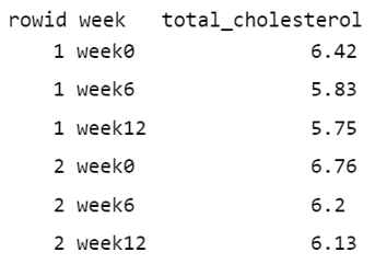
dat_TCH_long

# A tibble: 12 × 3
   rowid week   total_cholesterol
   <int> <chr>              <dbl>
 1     1 week0               6.42
 2     1 week6               5.83
 3     1 week12              5.75
 4     2 week0               6.76
 5     2 week6               6.2 
 6     2 week12              6.13
 7     3 week0               6.56
 8     3 week6               5.83
 9     3 week12              5.71
10     4 week0               4.8 
11     4 week6               4.27
12     4 week12              4.15

We observe that the “long” format consists of one column for the row ID, one for the week of measurement, and another for the total cholesterol values.

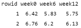
To better understand the dataset transformation from a “wide” to a “long” format, it’s helpful to break down the code and use data from the first two individuals (FIGURE 10.4).

FIGURE 10.4 Data of the first two participants in the “wide” format.

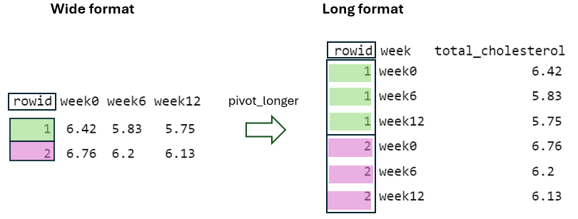
Initially, the cols = starts_with("week") argument specifies which columns from the original data should be pivoted. In this case, it selects the columns that start with the prefix “week”, such as “week0”, “week6”, and “week12”. Additionally, the values in the identifier column (rowid) in the “wide” format are repeated in the “long” format as many times as the number of columns being pivoted, which in this case is three (FIGURE 10.5).

FIGURE 10.5 The values of the identifier column (rowid) of “wide” format are repeated in the “long” format.

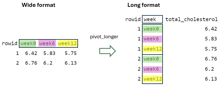
Next, by using the names_to = "week" argument, the column names being pivoted (i.e., week0, week6, and week12) become values within a newly defined variable, week, in the “long” format. These values are repeated as many times as the number of rows in the “wide” format, in this case two, while considering the rowid (FIGURE 10.6).

FIGURE 10.6 The column names being pivoted become values within a newly defined variable in the “long” format.

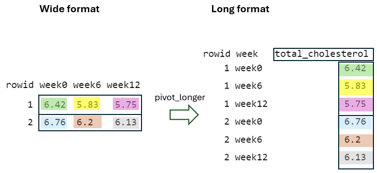
Finally, by using the values_to = "total_cholesterol" argument, the cell values from the pivoted variables are placed into a newly defined variable in the “long” format with the name total_cholesterol, with the rowid and week taken into account (FIGURE 10.7).

FIGURE 10.7 The cell values from the pivoted variables are placed into a newly defined variable in the “long” format.

 

10.5.2 From long to wide format

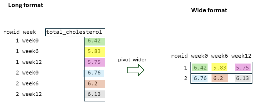
The pivot_wider() function is essentially the reverse of pivot_longer() function, reshaping data from “long” to “wide” format.

dat_TCH_wide <- dat_TCH_long |>
  pivot_wider(id_cols = rowid,
              names_from = week,
              values_from = total_cholesterol)
dat_TCH_wide

# A tibble: 4 × 4
  rowid week0 week6 week12
  <int> <dbl> <dbl>  <dbl>
1     1  6.42  5.83   5.75
2     2  6.76  6.2    6.13
3     3  6.56  5.83   5.71
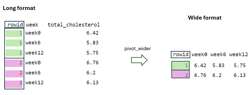
4     4  4.8   4.27   4.15

To better understand the reshaping process of the pivot_wider() function, let’s consider the data of the first two individuals in the “long” format (FIGURE 10.8):

FIGURE 10.8 Data of the first two participants in the “long” format.

First, in the “wide” format, the rowid column must contain unique values to ensure each row is uniquely identified within the dataset (FIGURE 10.9). This is achieved by using the argument id_cols = rowid, which specifies that the unique values from the rowid column in the “long” format should be used as the identifier column in the “wide” format.

FIGURE 10.9 The rowid values must be unique in the “wide” format.

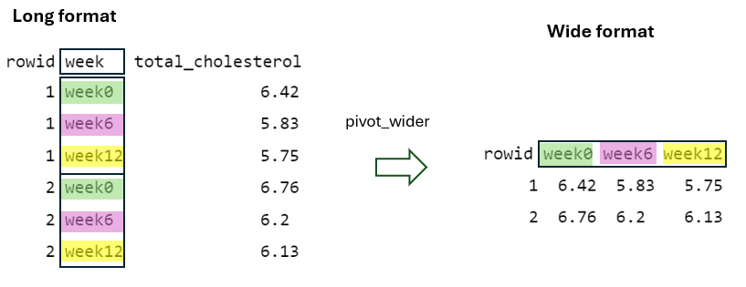
Second, the names_from = week argument specifies that the distinct week values in the “long” format serve as the basis for generating new column names (“week0”, “week6”, and “week12”) in the “wide” format (FIGURE 10.10).

FIGURE 10.10 New column names are generated from the distinct week values.

Finally, the values_from = total_cholesterol argument specifies that the total_cholesterol values of the “long” format must be placed into the cells of the new columns in the “wide” format, considering the rowid and week values (FIGURE 10.11).

FIGURE 10.11 The total cholesterol values are spread across the new columns in the “wide” format.

Altman, Douglas G, and J Martin Bland. 2007. “Missing Data.” BMJ 334 (7590): 424–24. https://doi.org/10.1136/bmj.38977.682025.2c.

Heymans, Martijn W., and Jos W. R. Twisk. 2022. “Handling Missing Data in Clinical Research.” Journal of Clinical Epidemiology 151 (November): 185–88. https://doi.org/10.1016/j.jclinepi.2022.08.016.